Implementation and examples — F-16 damage
This page describes the structure of the damage subsystem code and contains the worked examples. A short overview and quick start are on Aircraft damage modeling. All formulas are in Damage modeling mathematics.
Architecture and physical model
The implementation lives at
tensoraerospace/aerospacemodel/f16/nonlinear/damage/. A detailed design
document (outside the main navigation) is at
docs/superpowers/specs/2026-04-28-aircraft-damage-modeling-design.md —
available in the repository sources.
Key points:
- Parametric geometry recompute — at each damage event, mass, wing area, span, MAC, centre of gravity, and the inertia tensor are recomputed from per-section contributions using Huygens-Steiner.
- Strip-theory aerodynamic corrections — each section contributes proportionally to lost lift/drag/moment when damaged. Approximate fidelity ~10–20 % vs full vortex-lattice methods (VLM, Vortex Lattice Method) — adequate for RL training and quick FDM simulations, not for certification-grade modelling.
- Asymmetric damage requires the angular 6-DoF model with
split_stab=True(4-input action:[stab_left, stab_right, aileron,rudder]— separate channel per stabilator half plus combined ailerons and rudder). Symmetric damage works in both longitudinal and angular envs. - Bit-identical baseline — without a
damage_profile, env behaviour is byte-for-byte identical to the un-damaged baseline. Existing tests, trained agents, and saved trajectories work unchanged.
How the damage model works
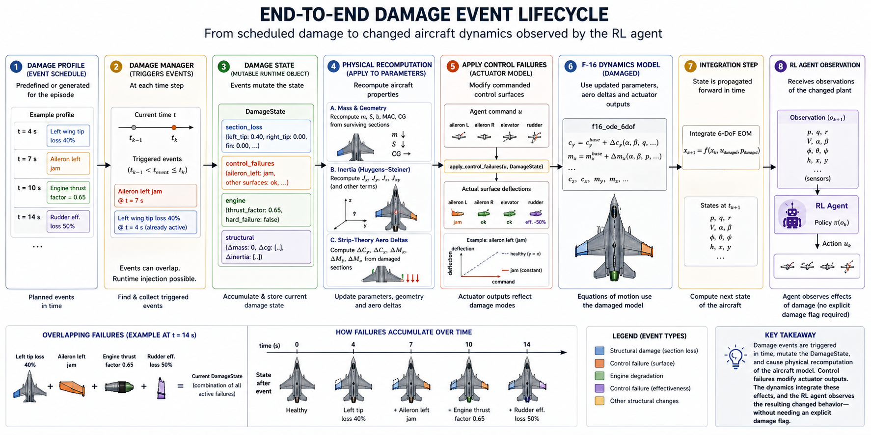
The damage subsystem turns the F-16 into a piecewise-time-varying plant. It does this with three linked layers: a section-based geometry, a damage state evolved by scheduled events, and a runtime physics recompute that feeds updated parameters and aero-coefficient deltas back into the existing F-16 ODEs.
The diagram below shows how a scheduled event flows through the entire
pipeline — from DamageProfile to the agent's observation:
Layer 1 — Section-based geometry
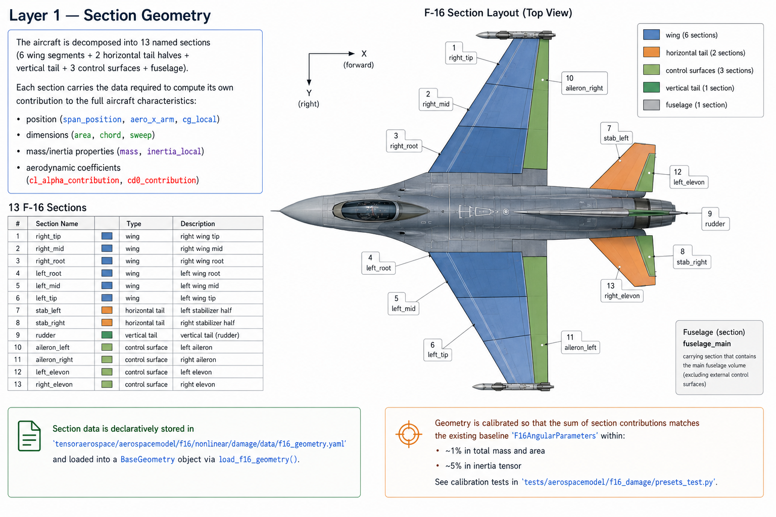
The aircraft is decomposed into 13 named sections (6 wing + 2 stabilator
halves + vertical tail + 3 control surfaces + fuselage). Each section
carries the data needed to compute its own contribution to the
aircraft-level totals: position (span_position, aero_x_arm, cg_local),
size (area, chord, sweep), inertial properties (mass, local
inertia_local), and aerodynamic coefficients (cl_alpha_contribution,
cd0_contribution).
The section data lives declaratively in
tensoraerospace/aerospacemodel/f16/nonlinear/damage/data/f16_geometry.yaml
and is loaded into a BaseGeometry object through load_f16_geometry().
Geometry is calibrated so that the sum of section contributions matches
the existing F16AngularParameters baseline within ~1 % for mass and
area, and ~5 % for the inertia tensor — see the calibration tests in
tests/aerospacemodel/f16_damage/presets_test.py.
Layer 2 — DamageState evolved by events
DamageState is a mutable runtime object describing the current health
of every section, every control surface, and the engine. It tracks four
sub-states:
section_loss: dict[str, float]— fraction in[0, 1]of each section that is missing.control_failures: dict[str, ControlFailure]— per-surface failure modes (jam,efficiency_loss,lost,free_floating).engine: EngineState—thrust_factorandhard_failureflag.structural: StructuralState— additional mass / CG / inertia deltas not tied to a specific section (e.g., dropped stores, ice accretion).
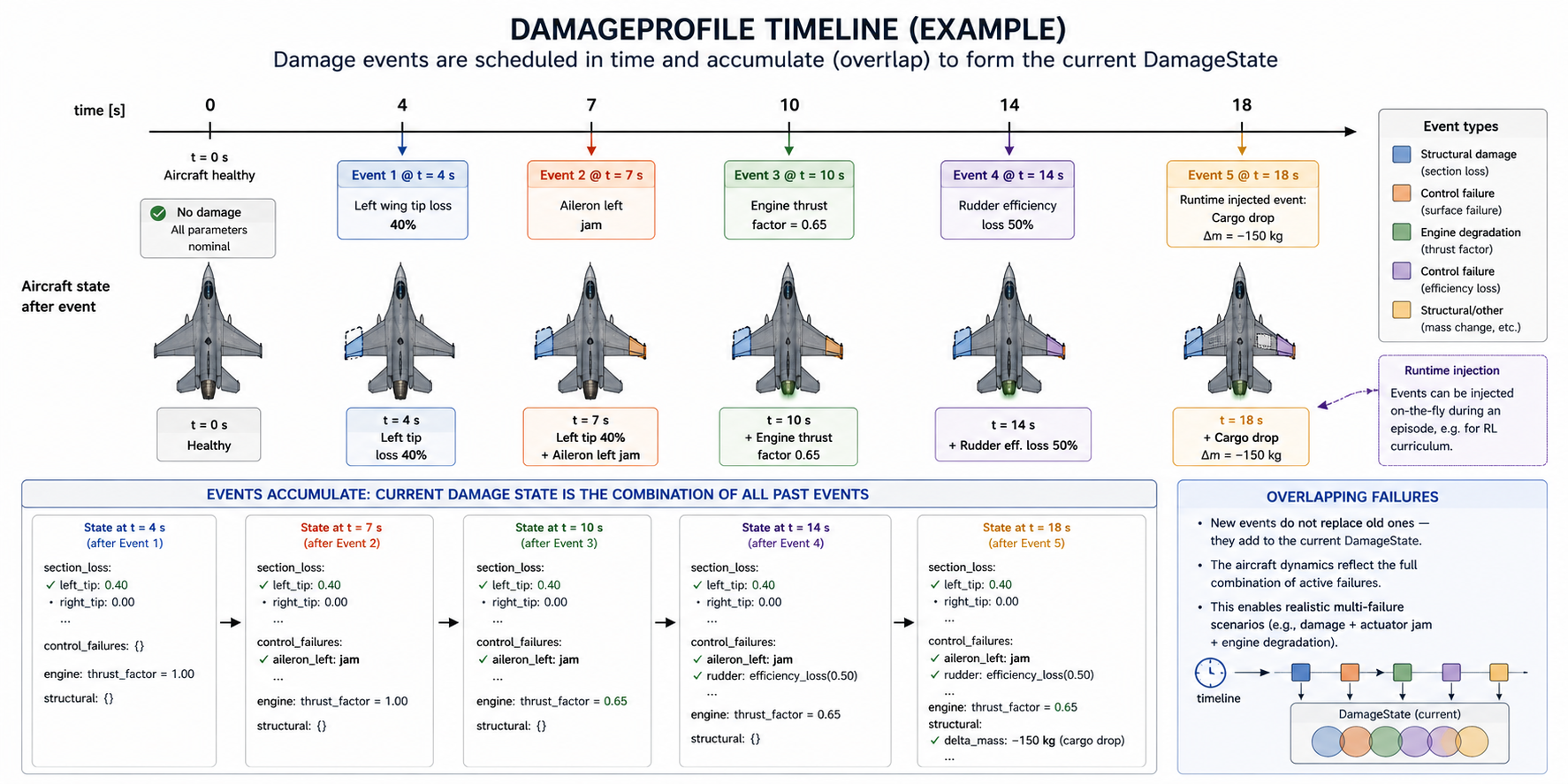
A DamageProfile is a list of DamageEvent entries each scheduled at a
specific trigger_time. The DamageManager (owned by the env) processes
the schedule on every step:
def update(self, t_current, t_previous):
    triggered = [
        e for e in self.profile.events
        if t_previous < e.trigger_time <= t_current
    ]
    for ev in triggered:
        self._apply_event(ev)        # mutates DamageState
    if triggered:
        apply_to_params(self.params, self.geometry, self.state)
    return triggered
Multiple events can stack (compound failures), and an injected one-shot
event can be added at runtime via damage_manager.inject_event(...) —
useful for RL curricula where damage is sampled per episode.
Layer 3 — Runtime physics recompute
When at least one event triggers, three physics computations run, in order (full formulas in the mathematics document):
(a) Mass-geometry recompute. Per-section masses scale by \((1 - f_s)\)
and the aircraft-level m, wing area S, span b, MAC bA, and CG
position are recomputed by mass-weighted aggregation. Symmetric tip loss
keeps the CG centred; asymmetric loss shifts it towards the surviving
side. See
Effective mass and centre of gravity
and Aerodynamic aggregates.
(b) Inertia recompute via Huygens-Steiner. For each surviving section with effective mass \(m^{eff}_s\), the parallel-axis theorem produces full \(J_{xx}, J_{yy}, J_{zz}, J_{xy}\) relative to the current aircraft CG. The \(J_{xy}\) (not \(J_{xz}\)) convention as the active off-diagonal is a deliberate body-frame choice in this F-16 model. Full derivation in Inertia tensor via Huygens-Steiner.
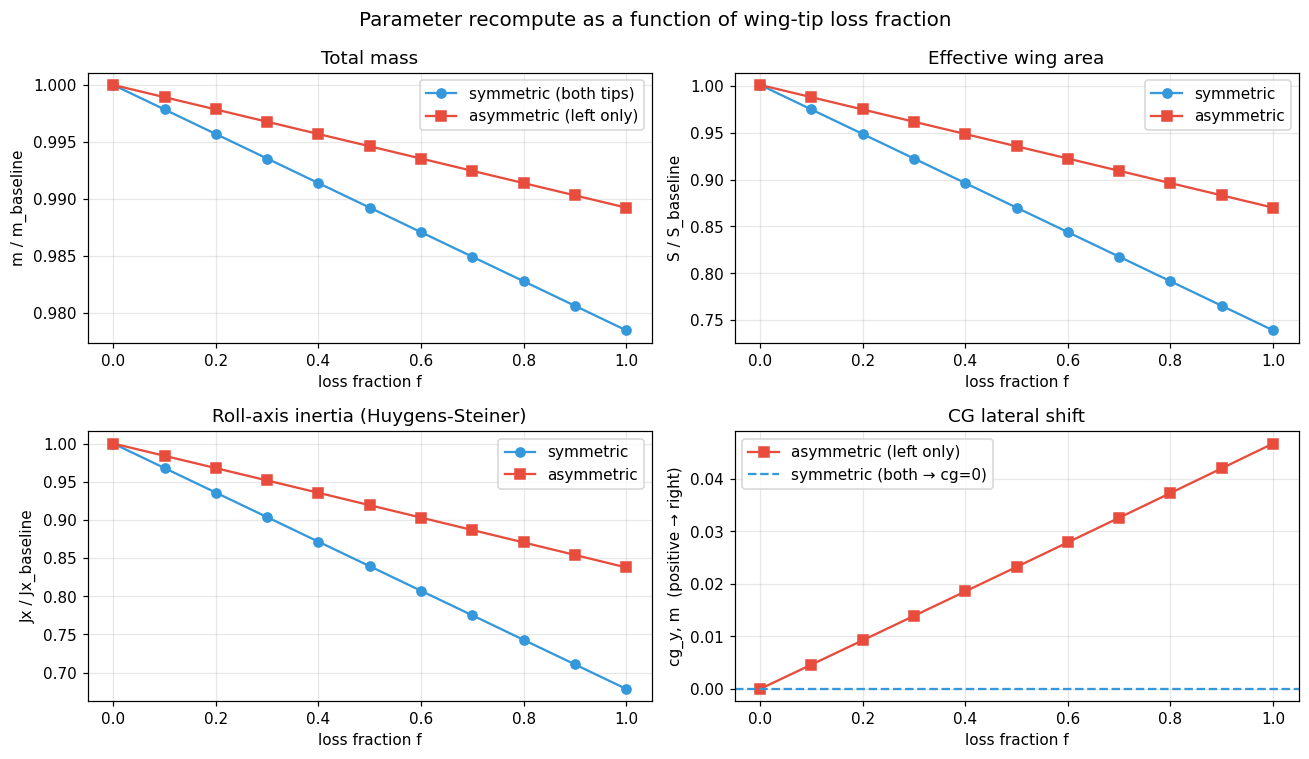
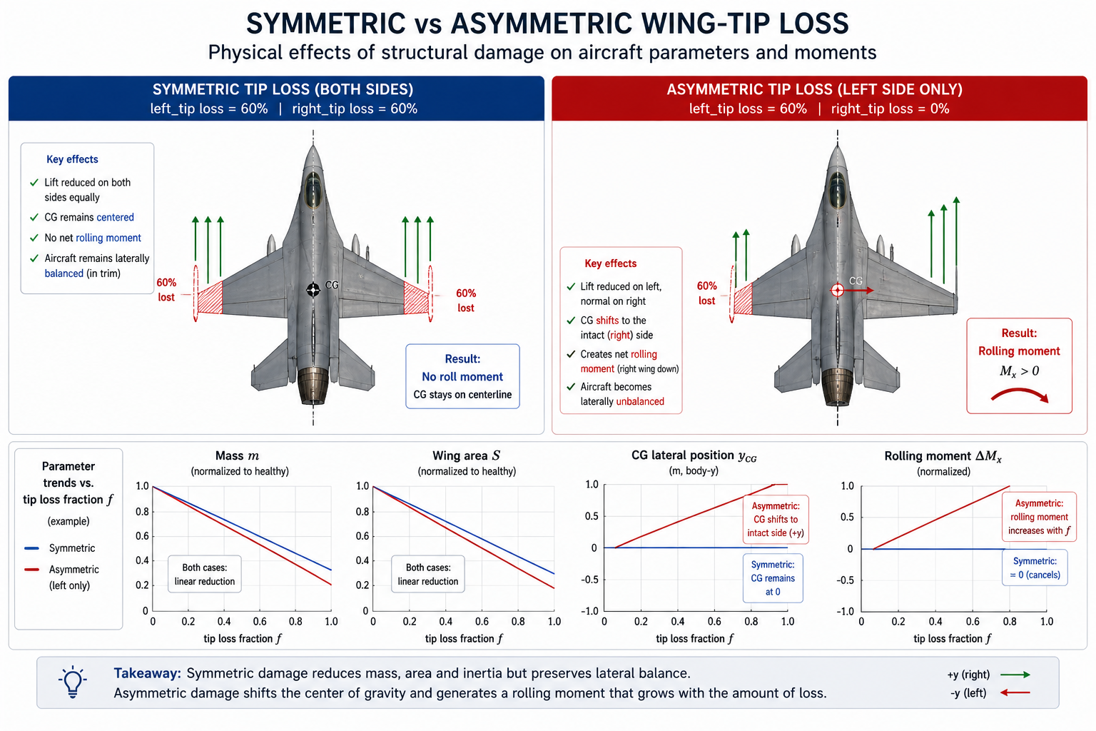
The plot above shows how m, S, Jx, and cg_y evolve as a function
of wing-tip loss fraction. Symmetric loss (blue) decays linearly without
disturbing the CG; asymmetric (red) introduces a CG shift that grows
with f.
(c) Strip-theory aerodynamic corrections. Each section contributes its own additive delta to the six aircraft-level coefficients on top of the baseline lookup tables: \(\Delta C_y, \Delta C_x, \Delta C_z, \Delta M_x, \Delta M_y, \Delta M_z\). Moment deltas include the section's lever arm, so losing a single tip produces a net rolling moment, while symmetric loss cancels. All formulas in Strip-theory aerodynamic deltas.
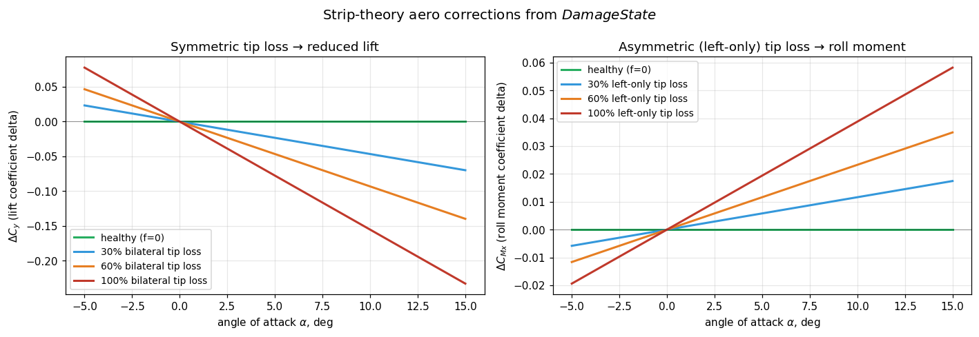
The two panels show this duality. Left: symmetric tip loss reduces
Cy proportionally — at α = 10° and 60 % bilateral loss, ΔCy ≈ -0.10,
i.e. ~12 % of the healthy lift. Right: asymmetric (left-only) loss
generates a roll-moment delta ΔMx that scales with both α and f —
this is the physics behind the dogfight scenario in
example/failure_demos/f16_damage_dogfight_demo.py.
The conceptual companion below collects the same physics into a single side-by-side comparison: symmetric loss preserves balance and only reduces lift, while asymmetric loss additionally introduces a CG shift and a rolling moment that grows with the loss fraction.
Putting it together — what the agent sees
Once damage is active, every step of the F-16 ODE picks up the corrections through a single hook:
# inside f16_ode_6dof
cy = get_cy(...) + delta_cy(α, β, geo, damage_state)
mx = get_mx(...) + delta_mx(α, β, geo, damage_state)
# ... etc for cx, cz, my, mz
Actuator commands also pass through apply_control_failures(u, state)
before reaching the integrator, so a jammed control surface produces a
non-trivial output independent of the agent's command. The agent therefore
does not need any explicit damage-state input: the dynamics it observes
are the damaged plant.
Visual companion — the 3D web viewer
The same flight log structure that drives the analytics plots also
feeds an interactive WebGL viewer. With render_mode="3d_web" on the
env, calling env.render() after the episode opens a self-contained
HTML in the browser (or returns inline HTML in Jupyter):
env = NonlinearAngularF16(..., render_mode="3d_web", damage_profile=profile)
env.reset()
for _ in range(N):
    env.step(action)
env.render()  # → browser tab or Jupyter cell
See Recipe 16 — Interactive 3D viewer for a walkthrough.
Worked example — wing tip loss in flight
example/failure_demos/f16_damage_dogfight_demo.py runs the angular F-16 with
damage_profile=WING_STRIKE_LEFT_TIP (full loss of left_tip at
t = 10 s). With zero stick command, the trajectory shows the asymmetry
clearly — pre-damage the aircraft holds straight-and-level; post-damage
a roll moment develops and ω_x grows to several deg/s within seconds.
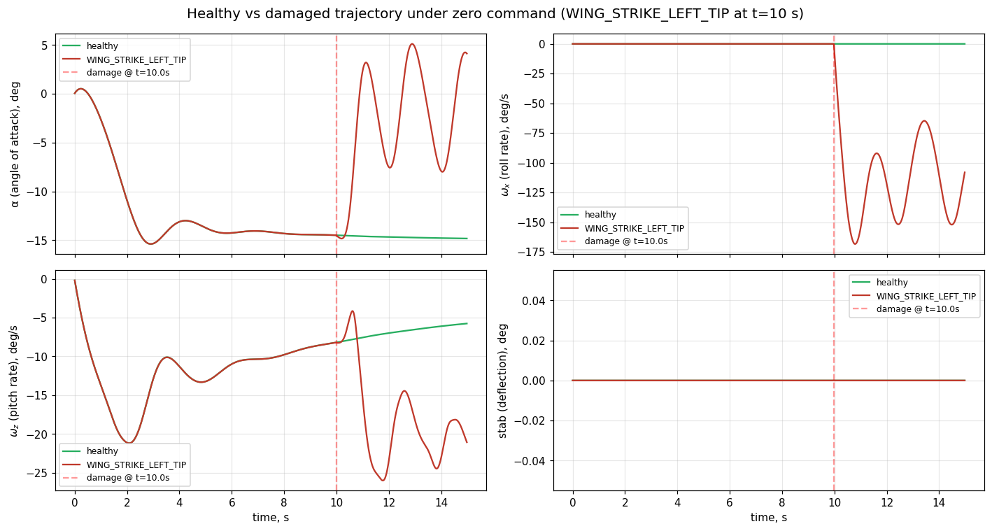
The roll-rate ω_x panel is the most direct demonstration: in the healthy
run it stays at zero, but after t = 10 s the damaged run accelerates —
this is exactly the moment imbalance produced by delta_mx in the
strip-theory layer. Pitch-rate ω_z and elevator stay in their pre-damage
ranges because the loss is not coupled to the pitch axis. The α channel
shows a small drift as the lift coefficient decreases.
Built-in scenarios
Seven ready-to-use DamageProfile constants, importable directly from
tensoraerospace.aerospacemodel.f16.nonlinear.damage:
| Preset | Trigger | Effect |
|---|---|---|
WING_STRIKE_LEFT_TIP |
t=10 s | Full loss of left wingtip |
WING_STRIKE_LEFT_HALF |
t=10 s | Left tip + 50% mid-section |
ELEVATOR_JAM_NEUTRAL |
t=5 s | Both stabilator halves jammed at neutral |
ELEVATOR_JAM_PITCH_UP |
t=5 s | Both jammed at +10° |
RUDDER_LOST |
t=5 s | Rudder lost |
ENGINE_FLAMEOUT |
t=5 s | Engine flameout (thrust = 0) |
BIRDSTRIKE_COMPOUND |
t=5 s | 20% right wing + 70% engine loss |
AIDI presets (AIDI = Adaptive Incremental Dynamic Inversion)
The same module also exposes three parameterised functions reproducing
the failure scenarios from Ul Haq et al. 2026 ("Adaptive Incremental
Dynamic Inversion for damaged F-16 control") — they return a
configurable DamageProfile:
from tensoraerospace.aerospacemodel.f16.nonlinear.damage import (
    stab_efficiency_step,
    aileron_efficiency_loss_schedule,
    rudder_total_loss,
)

# Single-step efficiency loss on the (left) stabilator
# (mu = surviving fraction of effectiveness)
profile_a = stab_efficiency_step(t_inject=5.0, mu=0.25, surface="stab_left")

# Progressive efficiency-loss schedule on an aileron
profile_b = aileron_efficiency_loss_schedule(
    t_start=2.0, dt_between=1.0,
    levels=(1.0, 0.75, 0.5, 0.25, 0.0),
    surface="aileron_left",
)

# Complete rudder loss — the "worst case" preset from the paper
profile_c = rudder_total_loss(t_inject=10.0)
A ready-to-run example is in example/reinforcement_learning/incremental_adp/example_aidi_damage_f16.ipynb.
Custom scenarios
from tensoraerospace.aerospacemodel.f16.nonlinear.damage import (
    DamageEvent, DamageProfile,
)

profile = DamageProfile(events=[
    DamageEvent(8.0, "section_loss",
                payload={"section": "right_mid", "loss_fraction": 0.4},
                label="right_mid_40pct"),
    DamageEvent(15.0, "engine_failure",
                payload={"thrust_factor": 0.3}),
])
Each event is DamageEvent(trigger_time, event_type, payload, label=None, duration=None).
The label is used in info["damage_events_triggered"] and the log for
readability (defaults to event_type if unset). The duration field is
reserved for future temporal effects and is currently ignored — damage is
permanent.
Event types and payload
section_loss
loss_fraction ∈ [0, 1] (out-of-range values are clipped). Valid section
names for the F-16:
| Group | Section names |
|---|---|
| Wing (6) | left_root, left_mid, left_tip, right_root, right_mid, right_tip |
| Stabilator (2) | stab_left, stab_right |
| Vertical tail | vtail |
| Control surfaces | rudder, aileron_left, aileron_right |
| Fuselage | fuselage_main |
Note: the API accepts fuselage_main, but losing the fuselage is
physically meaningless (catastrophic mass loss). It exists primarily for
mass-balance calibration and is normally not used in scenarios.
control_failure
Valid surfaces: stab_left, stab_right, aileron_left,
aileron_right, rudder. Valid modes:
| Mode | Extra payload fields | Effect |
|---|---|---|
jam |
jam_position_rad: float |
Surface frozen at the given position (rad), agent commands ignored |
efficiency_loss |
efficiency: float ∈ [0, 1] |
Command multiplied by efficiency |
lost |
— | Surface unresponsive (output = 0) |
free_floating |
— | Same as lost (output = 0) |
engine_failure
thrust_factor ∈ [0, 1] is the thrust multiplier; hard_failure=True
forces zero thrust regardless of the multiplier. Both fields are optional
(supply only one if needed).
structural_change
payload = {
    "mass_delta_kg": float,
    "cg_shift_m": tuple[float, float, float],
    "inertia_delta": tuple[float, float, float, float],  # ΔJx, ΔJy, ΔJz, ΔJxy
}
All fields are optional and applied additively (multiple events accumulate). Used for effects not tied to a specific section: store release / drops, ice accretion, fuel burn.
Runtime event injection
In addition to a pre-loaded DamageProfile, you can inject one-shot
events at runtime — useful for curriculum RL. The trigger_time is
absolute simulation time (since episode start):
from tensoraerospace.aerospacemodel.f16.nonlinear.damage import DamageEvent

# In a callback or training loop, t_now is the current sim time
event = DamageEvent(
    trigger_time=t_now + 0.5,            # fires 0.5 s from now
    event_type="section_loss",
    payload={"section": "left_tip", "loss_fraction": 0.5},
    label="injected_left_tip",
)
env.unwrapped.damage_manager.inject_event(event)
Injected events are single-fire and removed from the queue once they trigger.
Random profiles for RL
from tensoraerospace.aerospacemodel.f16.nonlinear.damage import (
    RandomDamageProfileGenerator,
)

generator = RandomDamageProfileGenerator(
    event_types=["section_loss", "control_failure", "engine_failure"],
    time_range=(5.0, 25.0),
    severity_range=(0.1, 1.0),
    num_events_range=(1, 2),
    seed=42,
    sections=("left_tip", "right_tip", "stab_left", "stab_right"),  # optional
)

profile = generator.sample()
obs, info = env.reset(options={"damage_profile": profile})
Constructor parameters:
event_types: list[str]— which event types are eligible for sampling ("section_loss","control_failure","engine_failure").time_range: (float, float)— uniform range fortrigger_time.severity_range: (float, float)— range forloss_fractiononsection_loss(default(0.1, 1.0)).num_events_range: (int, int)— number of events per profile (default(1, 1)).sections: tuple[str, ...]— sections allowed forsection_loss. Default:("left_tip", "left_mid", "right_tip", "right_mid", "stab_left", "stab_right")— i.e. the "losable" wing and stabilator sections (no roots, vtail or fuselage).seed: int | None— for reproducibility.
For control_failure, surfaces and modes are sampled uniformly from a
built-in list; for efficiency_loss the coefficient is drawn from
\([0.2, 0.9]\), for jam from \([-0.15, 0.15]\) rad.
What the env returns in info
When damage_profile or damage_observable is active, the info dict
returned from env.step(action) (not from env.reset()) contains:
info["damage_state"]— full JSON snapshot of the currentDamageState(fieldssection_loss,control_failures,engine,structural). Populated on every step.info["damage_events_triggered"]— list of labels (label, falling back toevent_typeiflabel=None) for events that fired this step. Present only on steps where events fire.
The env also accumulates history in env.unwrapped.damage_events_log
(event chronology) and damage_state_log (state snapshots at change
points) — used by the 3D viewer and convenient for offline analysis.
Damage event callback
You can register a callback fired right after each event is applied (useful for TensorBoard / WandB logging):
def on_damage(event, state):
    print(f"[t={event.trigger_time}] {event.label or event.event_type}")

env = NonlinearAngularF16(
    ...,
    damage_profile=profile,
    damage_event_callback=on_damage,
)
Observable damage
By default the agent does not observe the damage state — it must infer
deterioration from the dynamics. Pass damage_observable=True to extend
the observation vector with the loss fractions of all sections
(including stabilator, vtail, control surfaces, and fuselage — 13 total
on the F-16) and the scalar engine.thrust_factor:
env = NonlinearAngularF16(
    initial_state=np.zeros(14),
    number_time_steps=2000,
    damage_profile=profile,
    damage_observable=True,
    split_stab=True,
)
Observation layout: [14 base state elements, f_s for each section ingeo.section_names() order, thrust_factor]. The 14 base elements are the
state vector of the angular 6-DoF F-16 (see
Nonlinear 6-DoF angular). With
track_altitude=True the base part grows from 14 to 16 and the total
becomes 16 + N_sections + 1. For the F-16 standard configuration this
is 14 + 13 + 1 = 28.
You can also enable damage_observable=True without a
damage_profile — the agent then sees zeros in the damage fields and
unity in thrust_factor, but the observation dimensionality stays the
same. Useful for training "universal" policies with fixed input
dimensionality.
Resetting damage between episodes
env.reset() clears all damage and re-baselines parameters. To override
the profile per episode:
This is the standard pattern for RL training with randomised damage.
Adaptive RL agents under damage
The repository ships two end-to-end examples that demonstrate online
adaptive RL agents flying a 60-second mission with a damage event injected
at t=20 s. Both use the same scenario — symmetric 30 % loss of both
wing tips, applied through the proper DamageProfile API — so they
provide a direct apples-to-apples comparison.
| Example | Path | Format |
|---|---|---|
| iADP (Incremental ADP) | example/reinforcement_learning/incremental_adp/example_iadp_damage_f16.py |
runnable script |
| ET-DHP (Event-Triggered DHP) | example/reinforcement_learning/incremental_adp/example_etdhp_damage_f16.py |
runnable script |
| ET-DHP (notebook version) | example/reinforcement_learning/incremental_adp/example_etdhp_damage_f16.ipynb |
Jupyter notebook |
| AIDI (Adaptive Incremental Inversion) | example/reinforcement_learning/incremental_adp/example_aidi_damage_f16.ipynb |
Jupyter notebook |
Common scenario
- Underlying env:
NonlinearLongitudinalF16-v0at the global trim(α* = +4.92°, δₑ* = -4.45°). - Reference: 0.8 °/s (iADP) or 3° (ET-DHP) sinusoidal command on pitch-rate / α with a 2 s warm-up.
- Damage profile:
DamageProfile(events=[
    DamageEvent(20.0, "section_loss",
                payload={"section": "left_tip", "loss_fraction": 0.30}),
    DamageEvent(20.0, "section_loss",
                payload={"section": "right_tip", "loss_fraction": 0.30}),
])
At t=20 s the env recomputes m, S, bA, Jx/Jy/Jz/Jxy from the
per-section contributions, and the longitudinal ODE picks up
\(\Delta C_y = -\sum_s C_{l\alpha,s}\,\alpha\,f_s\,A_s/S_{base}\)
from strip theory.
iADP — closed-form policy + RLS plant identifier
from tensoraerospace.aerospacemodel.f16.nonlinear.damage import (
    DamageEvent, DamageProfile,
)
from tensoraerospace.agent.iadp import IADPAgent, IADPConfig

profile = DamageProfile(events=[
    DamageEvent(20.0, "section_loss",
                payload={"section": "left_tip", "loss_fraction": 0.30}),
    DamageEvent(20.0, "section_loss",
                payload={"section": "right_tip", "loss_fraction": 0.30}),
])

env = gym.make(
    "NonlinearLongitudinalF16-v0",
    number_time_steps=6002,
    initial_state=[alpha_trim, 0.0, stab_trim, 0.0],
    reference_signal=...,
    state_space=["alpha", "wz", "stab", "dstab"],
    control_space=["stab"],
    use_reward=False,
    dt=0.01,
    integrator="euler",
    control_bias=stab_trim_deg,
    damage_profile=profile,
).unwrapped
iADP (Incremental Approximate Dynamic Programming) uses a fixed-forgetting RLS (Recursive Least Squares) to track the local incremental plant \(\tilde{F}, \tilde{G}\) online, then derives the optimal control in closed form:
Because the RLS sees the new plant through the residuals as soon as the damage fires, \(\tilde{G}\) settles within tens of milliseconds — no fault detection or mode switching is required.
Sample run output:
=== Baseline (no damage) ===
Pre-damage RMSE  (5 s ≤ t < 20 s):  0.0701 °/s
Post-damage RMSE (22 s ≤ t ≤ 60 s): 0.0663 °/s

=== With damage (30% bilateral wing-tip loss at t=20s) ===
Pre-damage RMSE  (5 s ≤ t < 20 s):  0.0701 °/s
Post-damage RMSE (22 s ≤ t ≤ 60 s): 0.0703 °/s   ← negligible degradation
G̃ at t = 19.5 s: -0.00013                        ← pre-damage gain
G̃ at t = 25.0 s: -0.00017                        ← RLS still converging
G̃ at t = end:    +0.00010                        ← new stable estimate
Damage events triggered:
  t=19.99s : left_tip_30pct_loss
  t=19.99s : right_tip_30pct_loss
The post-damage RMSE (0.0703 °/s) is essentially identical to the no-damage baseline (0.0663 °/s). iADP keeps tracking the sinusoidal command without fault detection — the RLS observes the new plant gain through the residuals and the closed-form policy adapts.
ET-DHP — event-triggered actor/critic with frozen plant NN
from tensoraerospace.agent.et_dhp import ETDHPAgent, ETDHPConfig

cfg = ETDHPConfig(
    actor_hidden=(24, 24), critic_hidden=(24, 24), model_hidden=(24, 24),
    Q=[10.0, 0.1, 0.0, 0.0], R=[1.0], gamma=0.95,
    u_bound=2.0, rho=0.2, trigger_floor=0.1,
    seed=0,
)
agent = ETDHPAgent(n_state=4, n_control=1,
                   state_transform=state_transform, config=cfg)
agent.fit_plant_model(states_arr, actions_arr, next_states_arr)  # offline
ET-DHP (Event-Triggered Dual Heuristic Programming) uses three neural networks: a plant model, an actor, and a costate critic. The plant model is pre-trained offline on the healthy aircraft and frozen. A Lipschitz event trigger fires actor/critic updates only when the tracking error breaches a threshold.
Sample run output:
=== Baseline (no damage) ===
Pre-damage  (5–20 s):    MAE=0.094°  RMSE=0.114°
Post-damage (22–60 s):   MAE=0.166°  RMSE=0.235°
Triggers:                56 pre, 261 post

=== With damage (30% bilateral wing-tip loss at t=20s) ===
Pre-damage  (5–20 s):    MAE=0.210°  RMSE=0.268°
Post-damage (22–60 s):   MAE=0.702°  RMSE=0.913°   ← ~4× degradation
Triggers:                219 pre, 547 post           ← 2× rise after damage
Damage events:
  t=19.99s : left_tip_30pct_loss
  t=19.99s : right_tip_30pct_loss
Post-damage tracking degrades to ~0.9° RMSE (vs ~0.24° no-damage). The
event trigger correctly responds to the new plant — trigger count
roughly doubles after t=20 s — but the actor/critic alone cannot fully
compensate because the frozen plant NN's Jacobians F = ∂f/∂x,
G = ∂f/∂u no longer match the damaged dynamics.
iADP vs ET-DHP under damage — side by side
| iADP | ET-DHP | |
|---|---|---|
| Plant model | RLS, online | Neural network, frozen offline |
| Adaptation latency | ~10 ms (one RLS update) | Episodes (actor/critic gradient steps) |
| Detection signal | \(\tilde{G}\) shift in RLS | Trigger-count surge |
| Post-damage RMSE | ≈ baseline (no degradation) | ~4× baseline |
| Trade-off | Strong on adaptation, requires PE warm-start (Persistence of Excitation — input must be sufficiently exciting) | Robust by design via event triggering, but plant NN must be re-fit on damaged data to recover full performance |
Possible extensions
- Online plant-NN updates for ET-DHP: re-run
agent.fit_plant_model(...)on a sliding window of recent transitions, effectively making the plant model online too. - Damage-conditioned policies: pass
damage_observable=Trueto the env so the agent's observation includes the per-section loss vector and engine thrust factor — the actor can then condition on the damage state directly. - Curriculum training: combine
RandomDamageProfileGeneratorwith a per-episodeenv.reset(options={"damage_profile": ...})to train an agent that has seen a distribution of damage scenarios.