Lesson 9 -- Environments and Simulations

1. Overview

TensorAeroSpace ships a collection of Gymnasium-compatible environments for longitudinal control of aircraft, rockets and satellites. Every environment follows the standard gym.Env interface (reset, step, render) and can be instantiated either by class name or via gym.make(env_id).

There are two families of environments:

Family	Naming convention	Obs/act spaces	Reward	Intended use
Legacy	LinearLongitudinal*	raw physical units, 2-D column vectors (n, 1)	negative MSE	Classical control, IHDP, PID research
Improved	Improved* / *Normalized	normalized [-1, 1], flat 1-D vectors	LQR-style shaped reward with termination	RL training (PPO, SAC, TD3, ...)

Rule of thumb: use Legacy environments when you need direct access to the state-space model and physical units. Use Improved environments when training a neural-network policy.

---

2. Full Environment Catalogue

2.1 Legacy environments

Env ID	Class	Vehicle	Default states	obs dim	act dim
LinearLongitudinalB747-v0	LinearLongitudinalB747	Boeing 747	theta, q	2	1
LinearLongitudinalF16-v0	LinearLongitudinalF16	F-16 Fighting Falcon	alpha, q	2	1
LinearLongitudinalF4C-v0	LinearLongitudinalF4C	F-4C Phantom II	theta, q, alpha, V	4	1
LinearLongitudinalX15-v0	LinearLongitudinalX15	X-15 experimental	theta, q	2	1
LinearLongitudinalUAV-v0	LinearLongitudinalUAV	Generic UAV	theta, q	2	1
LinearLongitudinalUltrastick-v0	LinearLongitudinalUltrastick	Ultrastick-25e	theta, q	2	1
LinearLongitudinalLAPAN-v0	LinearLongitudinalLAPAN	LAPAN aircraft	theta, q	2	1
LinearLongitudinalELVRocket-v0	LinearLongitudinalELVRocket	ELV rocket	w, q, theta	3	1
LinearLongitudinalMissileModel-v0	LinearLongitudinalMissileModel	Missile	theta, q	2	1
GeoSat-v0	GeoSatEnv	Geostationary satellite	rho, theta, omega	3	1
ComSat-v0	ComSatEnv	Communication satellite	rho, rho_dot, theta_dot	3	1

2.2 Improved (RL-ready) environments

Env ID	Class	Vehicle	obs dim	act dim
ImprovedB747-v0	ImprovedB747Env	Boeing 747	4	1
ImprovedX15-v0	ImprovedX15Env	X-15	4	1
ImprovedELV-v0	ImprovedELVEnv	ELV rocket	4	1
ImprovedLAPAN-v0	ImprovedLAPANEnv	LAPAN aircraft	4	1
ImprovedMissile-v0	ImprovedMissileEnv	Missile	4	1
ImprovedComSat-v0	ImprovedComSatEnv	Comm. satellite	4	1
ImprovedUltrastick-v0	ImprovedUltrastickEnv	Ultrastick-25e	5	2
F4CPitchNormalized-v0	F4CPitchEnvNormalized	F-4C Phantom II	4	1

---

3. Legacy Environments in Depth

3.1 State-space model

Every legacy environment wraps a discrete linear model of the form:

x(t+1) = A x(t) + B u(t)
y(t)   = C x(t)

where x is the state vector, u is the control input (elevator deflection, thrust, etc.) and y is the measured output. Matrices A, B, C are loaded from the corresponding aerospacemodel module.

3.2 Observation shape

Legacy environments return observations as 2-D column vectors with shape (n, 1), where n is the number of states. Keep this in mind when feeding observations into a neural network -- you may need to flatten them first.

3.3 Key parameters

Parameter	Description
initial_state	Initial state vector (list of column vectors, e.g. [[0], [0]])
reference_signal	Target trajectory, shape (n_tracked, n_steps)
number_time_steps	Simulation horizon length
state_space	List of state variable names to observe
output_space	List of output variable names
tracking_states	Subset of states used for reward computation
reward_func	Optional custom reward callable
dt	Discretization time step (default 0.01 s)

3.4 Code example -- F-16 step tracking

import numpy as np
import gymnasium as gym
import matplotlib.pyplot as plt

from tensoraerospace.utils import generate_time_period, convert_tp_to_sec_tp
from tensoraerospace.signals.standard import unit_step

# Time grid
dt = 0.01
tp = generate_time_period(tn=20, dt=dt)
tps = convert_tp_to_sec_tp(tp, dt=dt)
number_time_steps = len(tp)

# 5-degree step reference for angle of attack, starting at t=5 s
reference = np.reshape(
    unit_step(degree=5, tp=tp, time_step=5, output_rad=True),
    [1, -1],
)

# Create environment
env = gym.make(
    "LinearLongitudinalF16-v0",
    number_time_steps=number_time_steps,
    initial_state=[[0], [0], [0]],
    reference_signal=reference,
    state_space=["theta", "alpha", "q"],
    output_space=["theta", "alpha", "q"],
    tracking_states=["alpha"],
)

obs, info = env.reset()

# Run simulation with zero control (open-loop)
states = [obs.flatten()]
for _ in range(number_time_steps - 1):
    action = np.array([[0.0]])  # no control input
    obs, reward, terminated, truncated, info = env.step(action)
    states.append(obs.flatten())
    if terminated or truncated:
        break

states = np.array(states)
time = np.array(tps[: len(states)])

# Plot angle of attack trajectory
plt.figure(figsize=(10, 5))
plt.plot(time, np.rad2deg(states[:, 1]), label="alpha (deg)")
plt.plot(time, np.rad2deg(reference[0, : len(time)]), "--r", label="reference")
plt.xlabel("Time (s)")
plt.ylabel("Angle of attack (deg)")
plt.title("F-16 open-loop response to step reference")
plt.legend()
plt.grid(True)
plt.show()

---

4. Improved Environments in Depth

4.1 Design principles

Improved environments are built specifically for RL training and share the following properties:

• Normalized spaces. Both observations and actions lie in [-1, 1]. The environment internally scales to/from physical units.
• Flat 1-D vectors. Observations are returned as (obs_dim,) arrays, not column vectors -- ready for standard policy networks.
• LQR-style shaped reward. The reward function is a weighted sum of tracking error, rate damping, control effort and smoothness terms.
• Safety termination. The episode terminates early (with a large negative penalty) if the vehicle exceeds physical limits such as maximum pitch angle or maximum pitch rate.

4.2 Walkthrough -- ImprovedB747Env

The ImprovedB747Env wraps the Boeing 747 longitudinal model with:

Component	Details
State vector	[u, w, q, theta] (velocity, vertical velocity, pitch rate, pitch angle) in SI units
Observation	[pitch_error, pitch_rate, pitch_angle, prev_action] -- all normalized to [-1, 1]
Action	Normalized elevator deflection, single float in [-1, 1] (maps to +/-25 deg)
Reward	-( w_pitch * e_pitch^2 + w_q * e_q^2 + w_action * |u| + w_smooth * |du| + w_jerk * |d2u| )
Termination	|theta| > 20 deg or |q| > 5 deg/s triggers penalty of -100
Truncation	Episode ends after number_time_steps

4.3 Constructor parameters

ImprovedB747Env(
    initial_state,                       # [u, w, q, theta] in SI
    reference_signal,                    # shape (1, n_steps), radians
    number_time_steps,                   # horizon
    dt=0.01,                             # time step (s)
    initial_elevator_deg=0.0,            # smooth start
    use_initial_action_on_first_step=True,
    reward_mode="step_response",         # or "tracking"
    survival_bonus=0.0,                  # per-step bonus for staying alive
    completion_bonus=0.0,                # bonus for finishing the episode
    early_termination_penalty=0.0,       # extra penalty on crash
    early_termination_penalty_per_step=0.0,
    include_reference_in_obs=False,      # adds 2 extra obs dims if True
)

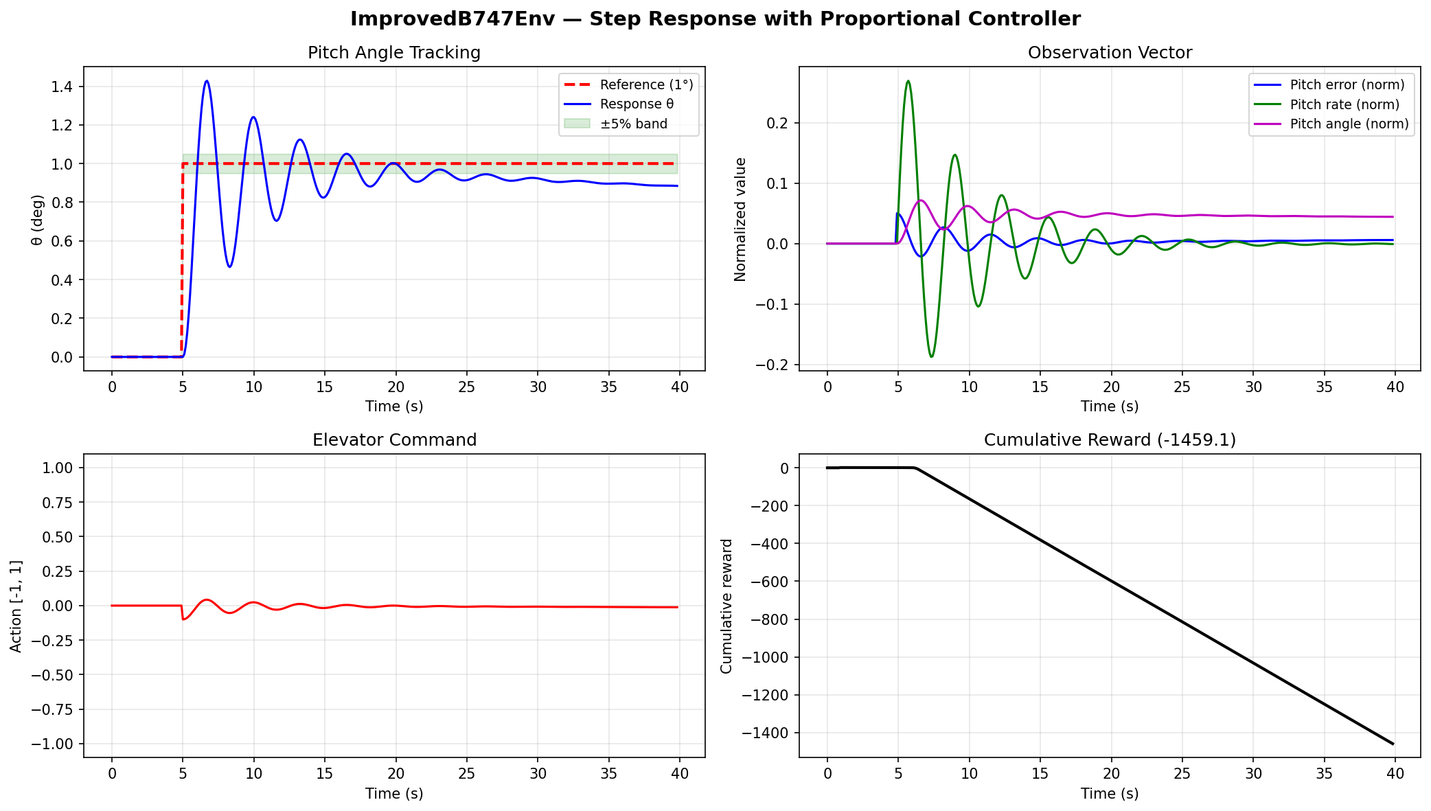
4.4 Code example -- proportional controller on B747

import numpy as np
import gymnasium as gym
import matplotlib.pyplot as plt

from tensoraerospace.utils import generate_time_period, convert_tp_to_sec_tp
from tensoraerospace.signals.standard import unit_step

dt = 0.01
tp = generate_time_period(tn=20, dt=dt)
tps = convert_tp_to_sec_tp(tp, dt=dt)
number_time_steps = len(tp)

# 3-degree pitch step at t=2 s
reference = np.reshape(
    unit_step(degree=3, tp=tp, time_step=2, output_rad=True),
    [1, -1],
)

env = gym.make(
    "ImprovedB747-v0",
    initial_state=[0.0, 0.0, 0.0, 0.0],
    reference_signal=reference,
    number_time_steps=number_time_steps,
    dt=dt,
)

obs, info = env.reset()

observations = [obs.copy()]
rewards = []
actions = []

for step in range(number_time_steps - 1):
    # Simple proportional control: action = -K_p * pitch_error
    # obs[0] is the normalized pitch error
    pitch_error = obs[0]
    action = np.array([-2.0 * pitch_error], dtype=np.float32)
    action = np.clip(action, -1.0, 1.0)

    obs, reward, terminated, truncated, info = env.step(action)
    observations.append(obs.copy())
    rewards.append(reward)
    actions.append(action[0])

    if terminated or truncated:
        break

observations = np.array(observations)
time = np.array(tps[: len(observations)])

fig, axes = plt.subplots(3, 1, figsize=(10, 10), sharex=True)

axes[0].plot(time, observations[:, 0], label="pitch error (norm)")
axes[0].set_ylabel("Normalized error")
axes[0].set_title("ImprovedB747Env -- Proportional controller")
axes[0].legend()
axes[0].grid(True)

axes[1].plot(time, observations[:, 2], label="pitch angle (norm)")
axes[1].set_ylabel("Normalized pitch")
axes[1].legend()
axes[1].grid(True)

axes[2].plot(time[: len(actions)], actions, label="action (norm)")
axes[2].set_xlabel("Time (s)")
axes[2].set_ylabel("Normalized action")
axes[2].legend()
axes[2].grid(True)

plt.tight_layout()
plt.show()

print(f"Episode length: {len(observations)} steps")
print(f"Total reward:   {sum(rewards):.2f}")

---

5. Reference Signals

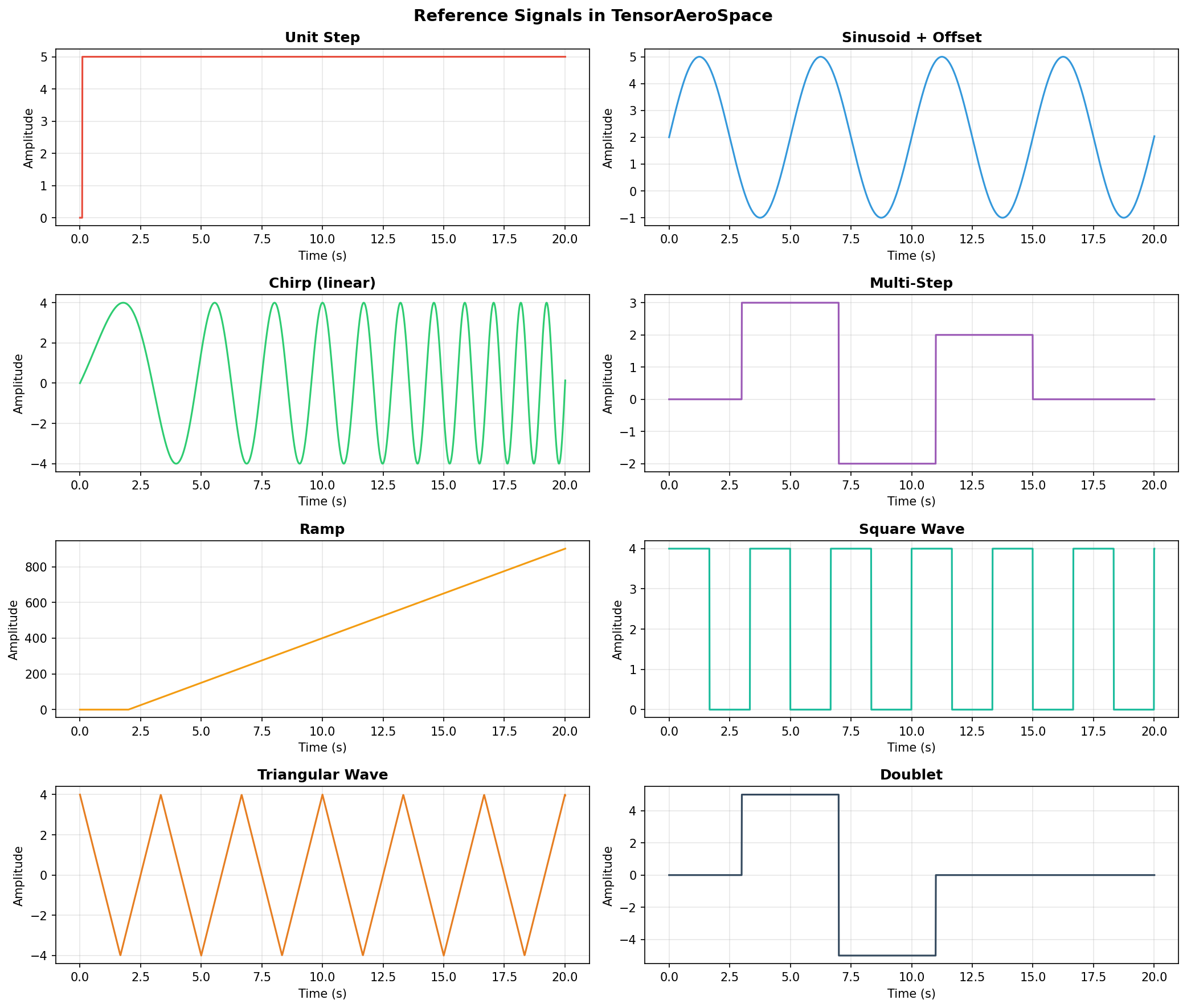
The module tensoraerospace.signals.standard provides ready-made reference signal generators for tracking tasks. All functions accept a time array tp (created by generate_time_period) and return a 1-D array of the same length.

5.1 Available signals

Function	Description	Key parameters
unit_step	Step function	degree, time_step, output_rad
sinusoid	Basic sine wave	frequency, amplitude
sinusoid_vertical_shift	Sine with DC offset	frequency, amplitude, vertical_shift
constant_line	Constant value	value_state
ramp	Linear ramp	slope, time_start
pulse	Rectangular pulse	amplitude, time_start, width
square_wave	Periodic square wave	frequency, amplitude, duty_cycle
sawtooth	Sawtooth wave	frequency, amplitude
triangular_wave	Triangular wave	frequency, amplitude
chirp	Frequency sweep	f0, f1, amplitude, method
doublet	Positive+negative pulse pair	amplitude, time_start, width
multi_step	Multiple step changes	step_times, step_values
exponential	Exponential approach	amplitude, time_constant, time_start
gaussian_pulse	Smooth bell pulse	amplitude, center, width
multisine	Sum of sinusoids	frequencies, amplitudes, phases
damped_sinusoid	Decaying oscillation	frequency, amplitude, damping

5.2 Code examples

import numpy as np
from tensoraerospace.utils import generate_time_period
from tensoraerospace.signals.standard import (
    unit_step, sinusoid_vertical_shift, chirp, multi_step, doublet
)

dt = 0.01
tp = generate_time_period(tn=20, dt=dt)

# Step signal: 5-degree step at t=3 s (output in radians)
sig_step = unit_step(tp=tp, degree=5, time_step=3, output_rad=True)

# Sinusoid with vertical offset
sig_sine = sinusoid_vertical_shift(
    tp=tp, frequency=0.2, amplitude=0.05, vertical_shift=0.05
)

# Chirp: frequency sweep from 0.1 Hz to 1.0 Hz
sig_chirp = chirp(tp=tp, f0=0.1, f1=1.0, amplitude=0.08)

# Multi-step: staircase reference
sig_multi = multi_step(
    tp=tp,
    step_times=[2, 6, 10, 15],
    step_values=[0.05, 0.03, -0.04, 0.02],
)

# Doublet: classic stability test maneuver
sig_doublet = doublet(
    tp=tp, amplitude=np.deg2rad(3), time_start=5.0, width=2.0
)

To use any signal as a reference for an environment, reshape it to (1, -1):

reference = np.reshape(sig_step, [1, -1])

---

6. Custom Environment Configuration

6.1 Changing simulation parameters

Both Legacy and Improved environments accept dt (time step) and number_time_steps (horizon). The total simulation time equals number_time_steps * dt.

# 30-second simulation at 50 Hz
dt = 0.02
tp = generate_time_period(tn=30, dt=dt)
number_time_steps = len(tp)

6.2 Custom initial states

For legacy environments, initial states are column vectors:

# F-16 with initial angle of attack of 2 degrees
initial_state = [[0], [np.deg2rad(2)], [0]]

For improved environments, states are flat arrays in SI units:

# B747 with small initial pitch rate
initial_state = [0.0, 0.0, np.deg2rad(0.5), 0.0]  # [u, w, q, theta]

6.3 Custom reward functions (Legacy environments)

Legacy environments accept a reward_func parameter. The function receives the current state, reference signal and time step:

def custom_reward(state, ref_signal, ts, action=None):
    """Penalize oscillation by adding a rate penalty."""
    if ref_signal.ndim == 2 and ref_signal.shape[1] > ts:
        ref_at_ts = ref_signal[:, ts].flatten()
    else:
        ref_at_ts = ref_signal.flatten()
    tracking_error = np.mean((state.flatten() - ref_at_ts) ** 2)
    rate_penalty = 0.1 * np.sum(state.flatten() ** 2)
    return float(-(tracking_error + rate_penalty))

env = gym.make(
    "LinearLongitudinalB747-v0",
    initial_state=[[0], [0]],
    reference_signal=reference,
    number_time_steps=number_time_steps,
    reward_func=custom_reward,
)

6.4 Reward modes in Improved environments

Improved B747 supports two reward modes:

• "step_response" (default) -- includes step-specific shaping terms for overshoot, settling time and oscillation. Best when training on step references.
• "tracking" -- universal mode using only base quadratic cost. Use for sinusoidal, chirp or other non-step reference signals.

env = gym.make(
    "ImprovedB747-v0",
    initial_state=[0.0, 0.0, 0.0, 0.0],
    reference_signal=reference,
    number_time_steps=number_time_steps,
    reward_mode="tracking",
)

---

7. Accessing Internal Model Data

Legacy environments expose the underlying aerospace model through env.unwrapped.model. This gives you access to state and control histories, as well as built-in plotting.

7.1 Key methods

Method	Description
model.get_state(name, to_deg=False)	Get state history as an array
model.get_control(name, to_deg=False)	Get control history as an array
model.plot_transient_process(name, time, ref, lang="eng", to_deg=True)	Plot state vs reference

7.2 Code example

import numpy as np
import gymnasium as gym
import matplotlib.pyplot as plt

from tensoraerospace.utils import generate_time_period, convert_tp_to_sec_tp
from tensoraerospace.signals.standard import unit_step

dt = 0.01
tp = generate_time_period(tn=20, dt=dt)
tps = convert_tp_to_sec_tp(tp, dt=dt)
number_time_steps = len(tp)

reference = np.reshape(
    unit_step(degree=5, tp=tp, time_step=5, output_rad=True),
    [1, -1],
)

env = gym.make(
    "LinearLongitudinalB747-v0",
    number_time_steps=number_time_steps,
    initial_state=[[0], [0]],
    reference_signal=reference,
    state_space=["theta", "q"],
    output_space=["theta", "q"],
    tracking_states=["theta"],
)

obs, _ = env.reset()
for i in range(number_time_steps - 1):
    action = np.array([0.5])  # constant elevator input
    obs, reward, terminated, truncated, info = env.step(action)
    if terminated or truncated:
        break

# Access the underlying model
model = env.unwrapped.model

# Retrieve state history
theta_deg = model.get_state("theta", to_deg=True)
q_deg = model.get_state("q", to_deg=True)

# Retrieve control history
stab_hist = model.get_control("stab", to_deg=True)

# Built-in plotting
model.plot_transient_process(
    "theta",
    time=np.array(tps),
    ref_signal=reference[0],
    lang="eng",
    to_deg=True,
    figsize=(10, 5),
)

---

8. Vectorized Environments

For efficient parallel training, ImprovedB747VecEnvTorch runs N independent B747 simulations in a single batched tensor operation. It supports both CPU and CUDA devices.

from tensoraerospace.envs import ImprovedB747VecEnvTorch

vec_env = ImprovedB747VecEnvTorch(
    num_envs=64,
    number_time_steps=2000,
    dt=0.01,
    device="cpu",        # or "cuda"
)

obs, info = vec_env.reset()
# obs shape: (64, 4) -- batch of 64 observations

for _ in range(2000):
    actions = vec_env.action_space_sample()  # random actions, shape (64, 1)
    obs, rewards, terminated, truncated, info = vec_env.step(actions)
    # rewards shape: (64,)

The vectorized environment also supports signal randomization -- automatically generating varied step, sine and ramp references for each sub-environment to prevent the agent from memorizing a single trajectory.

---

9. Environment Comparison

Env ID	Vehicle	obs	act	Reward	Termination	Recommended agents
LinearLongitudinalB747-v0	B747	2	1	-MSE	time limit	PID, IHDP, LQR
LinearLongitudinalF16-v0	F-16	2	1	-MSE	time limit	PID, IHDP, LQR
LinearLongitudinalF4C-v0	F-4C	4	1	-MSE	time limit	PID, IHDP, LQR
LinearLongitudinalX15-v0	X-15	2	1	-MSE	time limit	PID, IHDP, LQR
LinearLongitudinalUAV-v0	UAV	2	1	-MSE	time limit	PID, IHDP, LQR
LinearLongitudinalUltrastick-v0	Ultrastick	2	1	-MSE	time limit	PID, IHDP, LQR
LinearLongitudinalLAPAN-v0	LAPAN	2	1	-MSE	time limit	PID, IHDP, LQR
LinearLongitudinalELVRocket-v0	ELV	3	1	-MSE	time limit	PID, IHDP, LQR
LinearLongitudinalMissileModel-v0	Missile	2	1	-MSE	time limit	PID, IHDP, LQR
GeoSat-v0	GeoSat	3	1	-MSE	time limit	PID, LQR
ComSat-v0	ComSat	3	1	-MSE	time limit	PID, LQR
ImprovedB747-v0	B747	4	1	LQR-shaped	pitch/rate limits	PPO, SAC, TD3
ImprovedX15-v0	X-15	4	1	LQR-shaped	pitch/rate limits	PPO, SAC, TD3
ImprovedELV-v0	ELV	4	1	LQR-shaped	pitch/rate limits	PPO, SAC, TD3
ImprovedLAPAN-v0	LAPAN	4	1	LQR-shaped	pitch/rate limits	PPO, SAC, TD3
ImprovedMissile-v0	Missile	4	1	LQR-shaped	pitch/rate limits	PPO, SAC, TD3
ImprovedComSat-v0	ComSat	4	1	LQR-shaped	state limits	PPO, SAC, TD3
ImprovedUltrastick-v0	Ultrastick	5	2	LQR-shaped	pitch/rate limits	PPO, SAC, TD3
F4CPitchNormalized-v0	F-4C	4	1	LQR-shaped	pitch/rate limits	PPO, SAC, TD3

---

10. What's Next

In the next lesson we will use the Improved environments to train our first RL agent using PPO and SAC from the TensorAeroSpace agent library. We will learn how to configure hyperparameters, track training progress and evaluate the resulting autopilot against classical baselines.