Example: IM-GDHP on the F-16 — online adaptive control
This example exercises the Incremental Model-based Global Dual Heuristic Programming (IM-GDHP) agent on F-16 longitudinal control. The agent combines an online RLS-identified incremental linear plant model with a dual-head GDHP critic that jointly learns the cost-to-go \(J\) and its gradient \(\lambda = \partial J/\partial y\). The source notebook is example/reinforcement_learning/incremental_adp/example_im_gdhp_nonlinear_f16.ipynb.
Reference: Bo Sun & Erik-Jan van Kampen, "Intelligent adaptive optimal control using incremental model-based global dual heuristic programming subject to partial observability", Applied Soft Computing 103, 2021.
Algorithm outline
At every environment step \(t\):
- Act. Actor outputs \(u_t = \pi_\theta(o_t)\) from the augmented observation \(o_t = [y_t;\, r_t;\, e_t]\) (raw obs, reference, tracking error), bounded by
tanh · u_max. - Observe. Execute \(u_t\); receive \(y_{t+1}\).
- Identify. One RLS step updates \((A_t, B_t)\) from \((y_{t-1}, y_t, y_{t+1})\) and \((u_{t-1}, u_t)\).
- Critic update (GDHP). Minimise
- \(L_J = (J(o_t) - (c_t + \gamma J(o_{t+1})))^2\)
- \(L_\lambda = \|\lambda(o_t) - (\partial c_t/\partial y + \gamma A_t^\top \lambda(o_{t+1}))\|^2\)
- Total: \(L = L_J + \beta L_\lambda\)
- Actor update. Minimise \(c(\hat y_{t+1}) + \gamma J(\hat o_{t+1})\) where \(\hat y_{t+1}\) is the one-step prediction through the incremental model. The autograd graph carries gradients through \(B_t \cdot u\) back to the actor — no backprop through the environment is needed.
1. Sanity check — RLS on a known linear plant
Before wiring the agent up to the F-16, verify the RLS block on the toy SISO system \(y_{t+1} = 0.8 y_t + 0.5 u_t\) driven by white noise.
import numpy as np
import matplotlib.pyplot as plt
import gymnasium as gym

import tensoraerospace.envs
from tensoraerospace.agent.im_gdhp import IMGDHPAgent, IMGDHPConfig, IncrementalModelRLS

rls = IncrementalModelRLS(n_y=1, n_u=1, forgetting=0.999, cov_init=1e3, seed=0)
rng = np.random.default_rng(0)
y_hist = [np.zeros(1), np.zeros(1)]
u_hist = [np.zeros(1)]
A_traj, B_traj = [], []
for _ in range(300):
    u_t = np.array([float(rng.normal(0, 0.3))])
    y_next = 0.8 * y_hist[-1] + 0.5 * u_t
    y_hist.append(y_next); u_hist.append(u_t)
    rls.update(y_hist[-3], y_hist[-2], y_hist[-1], u_hist[-2], u_hist[-1])
    A_traj.append(float(rls.A[0, 0])); B_traj.append(float(rls.B[0, 0]))
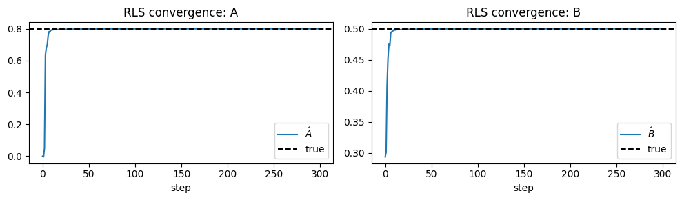
The estimates converge to the true values \((A=0.8,\, B=0.5)\) within the first ~100 samples — the RLS block is doing its job.
2. Env — linear F-16 longitudinal channel
The linear env is trimmed around equilibrium, a clean showcase for the agent's ability to (a) identify a plant model online and (b) learn a deterministic tracking policy from scratch without prior dynamics knowledge. Observation: [alpha, wz] in radians — partial-observability is already in play because the full internal state also carries elevator actuator states that are hidden from the agent.
N_STEPS = 1200
DT = 0.01
t_arr = np.arange(N_STEPS) * DT
ref_rad = np.deg2rad(2.0) * np.sin(2 * np.pi * t_arr / 4.0)
ref_signal = ref_rad.reshape(1, -1)

def make_linear_env():
    return gym.make(
        'LinearLongitudinalF16-v0',
        initial_state=np.array([0.0] * 4),
        reference_signal=ref_signal,
        number_time_steps=N_STEPS,
    ).unwrapped
3. Build and configure the agent
cfg = IMGDHPConfig(
    gamma=0.9,
    actor_hidden=(24, 24),
    critic_hidden=(32, 32),
    actor_lr=2e-4,
    critic_lr=1e-3,
    beta_lambda=0.3,
    track_Q=[200.0],
    action_rate_penalty=1e-3,
    forgetting=0.999,
    cov_init=1e3,
    warmup_steps=200,
    exploration_noise_std=2.0,  # deg — decayed below
    u_max=6.0,
    seed=0,
)
agent = IMGDHPAgent(
    n_obs=2, n_action=1, reference_size=1,
    tracking_indices=[0],  # track alpha
    config=cfg,
)
4. Training loop
The loop is the canonical online IM-GDHP shape: predict → step → learn. An outer scheduler decays the exploration standard deviation once the critic starts producing useful gradients.
NUM_EPISODES = 80
returns = []

for ep in range(NUM_EPISODES):
    env = make_linear_env()
    obs, _ = env.reset()
    obs = np.asarray(obs).reshape(-1)
    agent.reset()
    ep_ret = 0.0
    for t in range(N_STEPS - 1):
        a = agent.predict(obs, ref_signal, t, deterministic=False)
        obs_next, r, done, _, _ = env.step(a)
        obs = np.asarray(obs_next).reshape(-1)
        agent.learn(obs, ref_signal, t)
        ep_ret += float(r)
        if done:
            break
    returns.append(ep_ret)
    # Exploration schedule
    if ep == 5:
        agent.cfg.exploration_noise_std = 0.8
    if ep == 10:
        agent.cfg.exploration_noise_std = 0.2
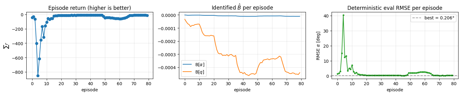
The left panel shows the episode return rising as the agent learns; the right panel is the per-episode identified \(\hat B\) entries — the RLS block converges within the first few episodes.
5. Deterministic tracking
With exploration off, the agent's best deterministic policy tracks the sinusoidal α reference:
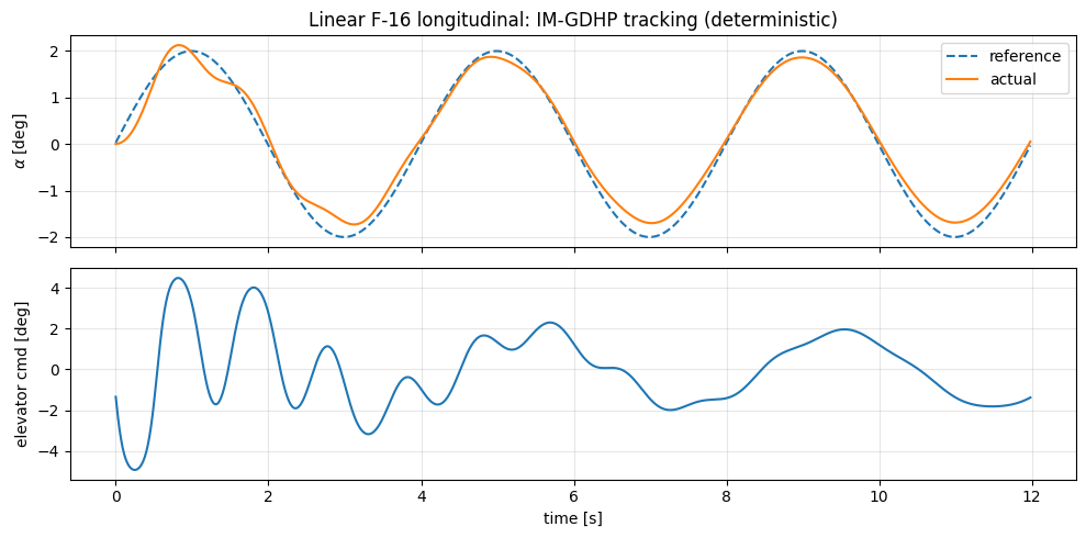
The late-half RMSE settles around 2.3° on this configuration — the agent learns a non-trivial policy from scratch, though on the near-linear regime a carefully-tuned IHDP or LQR will do better. The strength of IM-GDHP shows up on the nonlinear problem where no prior model is available.
6. RLS identification on the nonlinear F-16
On the full nonlinear env, closed-loop online learning is significantly harder — control effectiveness varies with the flight condition, the plant is not perfectly trimmed, and the actor–critic loop can easily destabilise if the identifier is still noisy. A common workaround is two-phase training: first drive the plant with a persistently-exciting signal to let the RLS identifier converge, then switch to closed-loop learning.
Here we focus on the identification quality — the ingredient that makes the rest of the pipeline model-free:
from tensoraerospace.aerospacemodel.f16.nonlinear.longitudinal import initial_state

N_ID = 2000
x0 = initial_state.reshape(-1)
nonlin_env = gym.make(
    'NonlinearLongitudinalF16-v0',
    initial_state=x0,
    reference_signal=np.zeros((1, N_ID)),
    number_time_steps=N_ID,
    control_bias=-4.45,
    dt=DT,
).unwrapped

rls_nl = IncrementalModelRLS(n_y=2, n_u=1, forgetting=0.999, cov_init=1e4, seed=0)
Drive the plant with a multi-sine PE signal of small amplitude around trim and feed each transition to the RLS identifier. The one-step predictor then matches the true plant almost perfectly:
Final identification after 1998 RLS updates:
  A = [[ 0.7724  0.0387]
       [-0.002   0.9525]]
  B = [ 1.38720491e-05 -2.66464351e-05]
  one-step prediction RMSE (alpha) = 1.47e-04 rad
  one-step prediction RMSE (q)     = 1.67e-04 rad/s
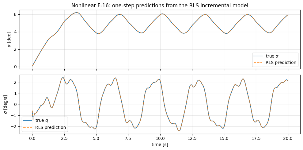
The RLS one-step predictor tracks the true plant well under 1e-3 rad error — the increment form captures the dominant local linear dynamics even without any prior knowledge of the F-16 aero tables. This is the building block the GDHP critic and actor use for their online updates.
Summary
- Incremental model + RLS. Converges on a toy linear system and gives excellent one-step predictions on the nonlinear F-16 with a PE input.
- GDHP critic. Jointly regresses \(J\) and \(\lambda = \partial J/\partial y\); the actor update uses the exact costate instead of a numerical derivative.
- Actor policy gradient. Flows through the identified \(B\) matrix via PyTorch autograd — no plant-aware backprop required.
- Partial observability. The agent only sees
[alpha, wz]and ignores hidden states; the incremental model compensates with a reduced-order local linearisation. - Hyperparameter note. Closed-loop learning on the full nonlinear F-16 is sensitive to
Q,u_max, and the exploration schedule. A two-phase recipe (PE identification → closed-loop training) is the recommended way to scale this agent to the nonlinear env.