Quadrotor: usage examples¶

Practical recipes for the tensoraerospace.aerospacemodel.quadrotor.nonlinear and tensoraerospace.aerospacemodel.quadrotor.damage modules. All snippets are self-contained — copy and run as-is. For the theoretical model description see Quadrotor (Nonlinear 6-DoF).

Nonlinear 6-DoF¶

1. Bare hover¶

The simplest case: the quadrotor is held at the origin by a constant thrust m·g. The RK4 integrator does this to machine precision.

import numpy as np

from tensoraerospace.aerospacemodel.quadrotor.nonlinear import NonlinearQuadrotor

m = NonlinearQuadrotor(x0=np.zeros(12), dt=0.01, integrator="rk4")
u_hover = np.array([m.hover_thrust, 0.0, 0.0, 0.0])  # T, τ_x, τ_y, τ_z

for _ in range(1000):  # 10 s
    m.run_step(u_hover)

print(f"max |state| after 10 s: {np.max(np.abs(m.current_state)):.2e}")
# → ≈ 0 (exact equilibrium)

2. Free fall (no thrust)¶

With zero thrust and linear drag the quadrotor approaches the terminal velocity v∞ = m·g / k_dz. Analytic solution:

\[ z(t) = v_\infty t + v_\infty \tau (e^{-t/\tau} - 1), \qquad \tau = m / k_{dz}. \]

import numpy as np

from tensoraerospace.aerospacemodel.quadrotor.nonlinear import NonlinearQuadrotor

m = NonlinearQuadrotor(x0=np.zeros(12), dt=0.001, integrator="rk4")
T_zero = np.zeros(4)

for _ in range(10_000):  # 10 s
    m.run_step(T_zero)

mass, g, k_dz = m.param.m, m.param.g, m.param.kdz
v_inf = mass * g / k_dz
tau = mass / k_dz
z_pred = v_inf * 10.0 + v_inf * tau * (np.exp(-10.0 / tau) - 1.0)

z_real = m.current_state[2]  # NED: positive z = down
print(f"z (model)     = {z_real:.3f} m")
print(f"z (analytic)  = {z_pred:.3f} m")
print(f"|delta|       = {abs(z_real - z_pred):.2e}")
# Match to 6+ decimals

3. Roll disturbance + P-feedback on phi¶

Start with a 3° roll and damp it with a simple proportional regulator on phi. A small KP_PHI = -0.05 gives near-critical damping at the default inertia.

import numpy as np

from tensoraerospace.aerospacemodel.quadrotor.nonlinear import (
    NonlinearQuadrotor,
    set_initial_state,
)

m = NonlinearQuadrotor(
    x0=set_initial_state(phi=np.deg2rad(3.0)),
    dt=0.005,
    integrator="rk4",
)

T_hover = m.hover_thrust
KP_PHI = -0.05
for _ in range(2000):  # 10 s
    phi = m.current_state[6]
    tau_x = KP_PHI * phi
    m.run_step(np.array([T_hover, tau_x, 0.0, 0.0]))

phi_final = np.rad2deg(m.current_state[6])
print(f"Final roll: {phi_final:+.4f}°  (started +3°)")

4. Integrator comparison: Euler vs RK4¶

At small dt both integrators converge to the same solution; at larger dt RK4 stays more accurate. Test: hover with a 0.5 N·m roll torque applied for 10 s.

import numpy as np

from tensoraerospace.aerospacemodel.quadrotor.nonlinear import NonlinearQuadrotor

DT = 0.05  # relatively coarse
N = 200    # 10 s

results = {}
for integ in ("euler", "rk4"):
    m = NonlinearQuadrotor(x0=np.zeros(12), dt=DT, integrator=integ)
    u = np.array([m.hover_thrust, 0.5, 0.0, 0.0])
    for _ in range(N):
        m.run_step(u)
    results[integ] = m.current_state

print(f"After 10 s with tau_x = 0.5 N·m:")
print(f"  Euler:  phi = {np.rad2deg(results['euler'][6]):.4f}°")
print(f"  RK4:    phi = {np.rad2deg(results['rk4'][6]):.4f}°")

5. Custom parameters (different mass, inertia, drag)¶

Replace default_parameters() with your own QuadrotorParameters to model a different airframe.

import numpy as np

from tensoraerospace.aerospacemodel.quadrotor.nonlinear import (
    NonlinearQuadrotor,
    QuadrotorParameters,
)

# Lightweight 250 g racing drone
custom = QuadrotorParameters(
    m=0.25,
    Jx=0.0008, Jy=0.0008, Jz=0.0015,
    arm_length=0.085,
    kdx=0.02, kdy=0.02, kdz=0.04,
    thrust_max=10.0,
)

m = NonlinearQuadrotor(x0=np.zeros(12), dt=0.005, integrator="rk4")
m.set_param(custom)

print(f"Hover thrust: {m.hover_thrust:.3f} N  (mass {m.param.m} kg)")
# 0.25·9.81 = 2.4525 N

6. Reading state and control history¶

ModelBase keeps the full trajectory; access it via get_state(name) and get_control(name) (with optional unit conversion).

import numpy as np
import matplotlib.pyplot as plt

from tensoraerospace.aerospacemodel.quadrotor.nonlinear import NonlinearQuadrotor

m = NonlinearQuadrotor(x0=np.zeros(12), dt=0.01, integrator="rk4")
T_hover = m.hover_thrust

# 0.2-s τ_x impulse
for k in range(500):
    tau_x = 0.3 if 100 <= k < 120 else 0.0
    m.run_step(np.array([T_hover, tau_x, 0.0, 0.0]))

phi_deg = m.get_state("phi", to_deg=True)
p_deg_s = m.get_state("p", to_deg=True)
tau_x_log = m.get_control("tau_x")

t = np.arange(len(phi_deg)) * m.dt
fig, axes = plt.subplots(3, 1, figsize=(9, 6), sharex=True)
axes[0].plot(t, tau_x_log); axes[0].set_ylabel(r"$\tau_x$, N·m")
axes[1].plot(t, p_deg_s);  axes[1].set_ylabel(r"$p$, °/s")
axes[2].plot(t, phi_deg);  axes[2].set_ylabel(r"$\varphi$, °")
axes[2].set_xlabel("time, s")
plt.tight_layout(); plt.show()

Companion notebook: `example_ihdp_quadrotor.ipynb`¶

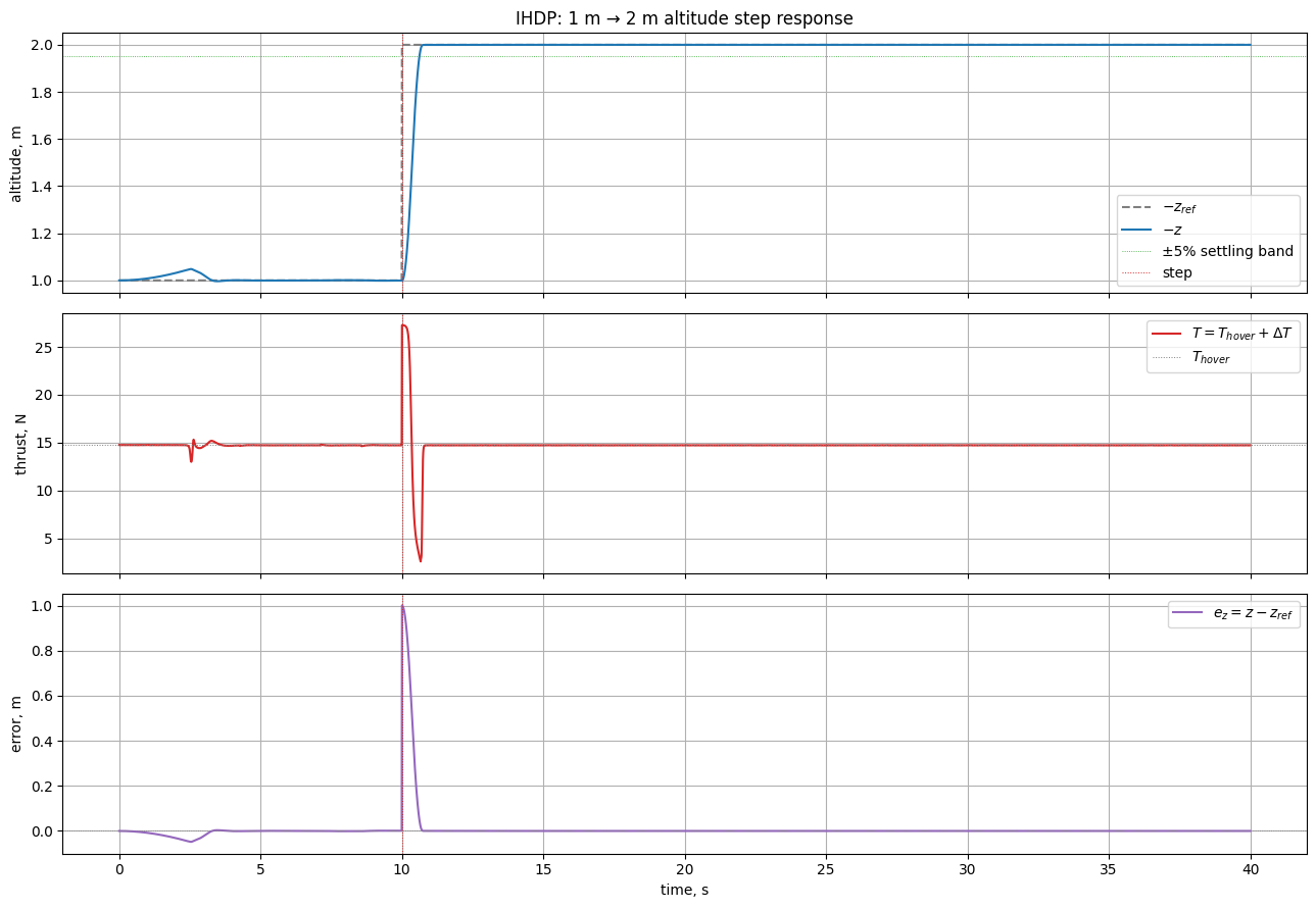
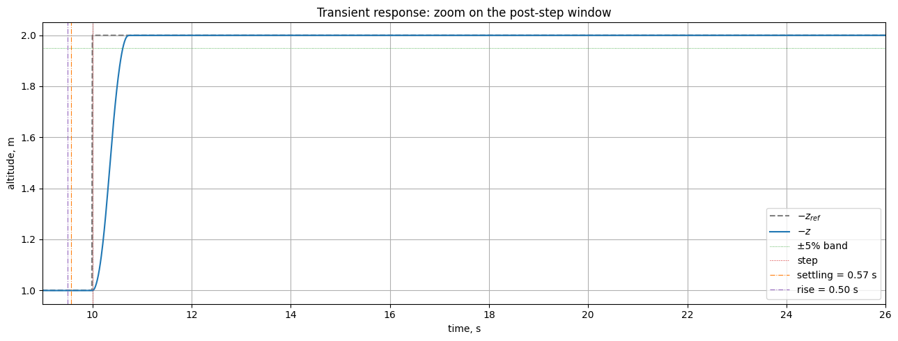
The same PD altitude tracking scenario extended to a full step response with IHDP, evaluated by ControlBenchmark. Reference: 1 m → 2 m at t = 10 s.

Zoom on the transient with rise_time and settling_time markers:

7. PD altitude tracking — climb to 2 m¶

Hover mode extended with PD feedback on (z, w_b). With attitude held level the full quadrotor reduces to a near-linear vertical system.

import numpy as np

from tensoraerospace.aerospacemodel.quadrotor.nonlinear import NonlinearQuadrotor

m = NonlinearQuadrotor(x0=np.zeros(12), dt=0.01, integrator="rk4")
T_hover = m.hover_thrust
mass = m.param.m

z_ref = -2.0  # NED: target altitude 2 m above starting plane
KP, KD = 6.0, 6.0  # PD on (e_z, w_b)

def attitude_torques(state):
    phi, theta = state[6], state[7]
    p, q, r = state[9], state[10], state[11]
    return np.array([
        -0.05 * p - 0.30 * phi,
        -0.05 * q - 0.30 * theta,
        -0.05 * r,
    ])

for _ in range(800):  # 8 s
    s = m.current_state
    e_z = s[2] - z_ref
    dT = mass * (KP * e_z + KD * s[5])
    T = T_hover + np.clip(dT, -10.0, 10.0)
    m.run_step(np.array([T, *attitude_torques(s)]))

print(f"Final altitude: {-m.current_state[2]:.4f} m (target 2.0 m)")

Damage subsystem¶

Companion notebook: `example_etdhp_quadrotor_damage.ipynb`¶

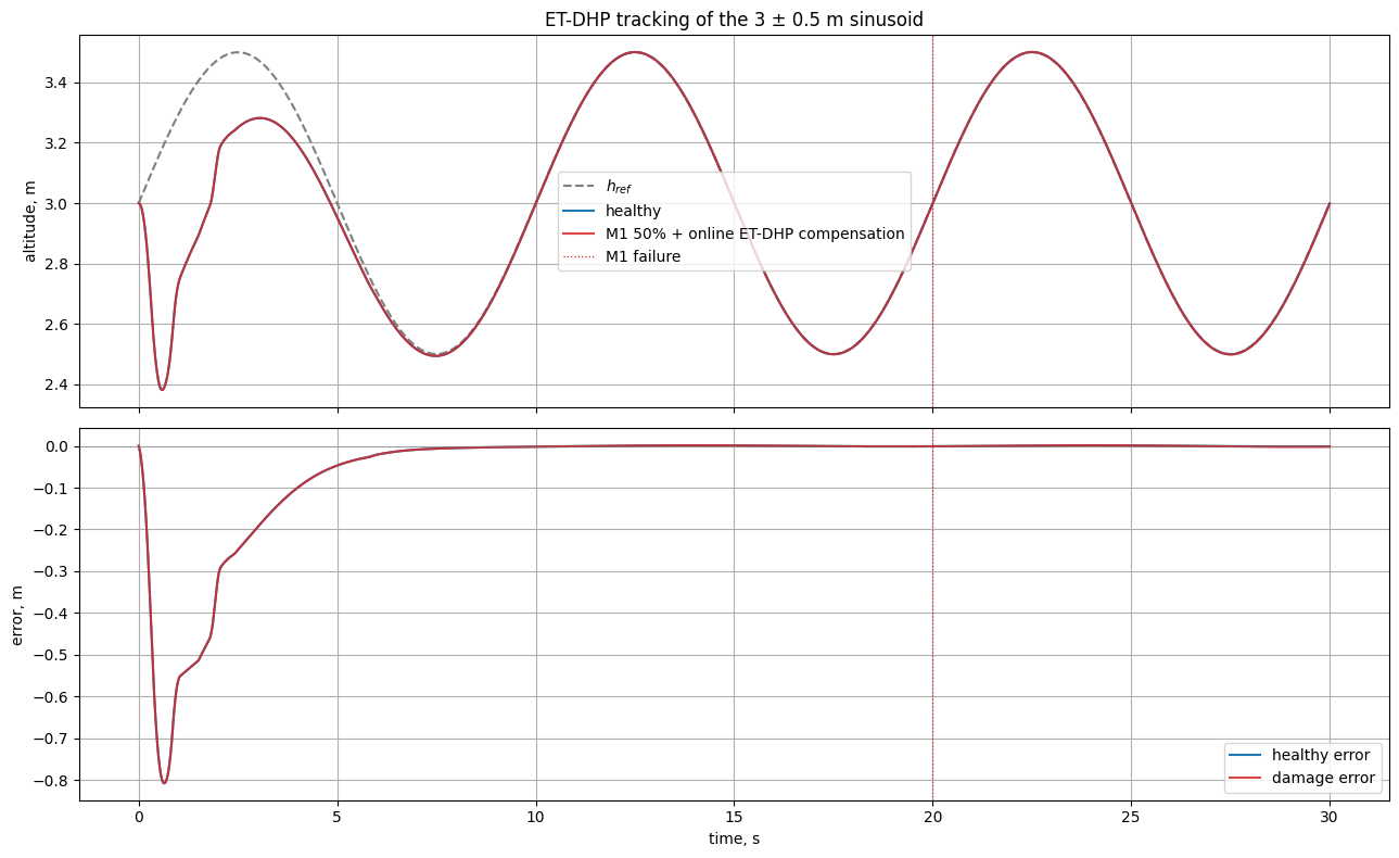
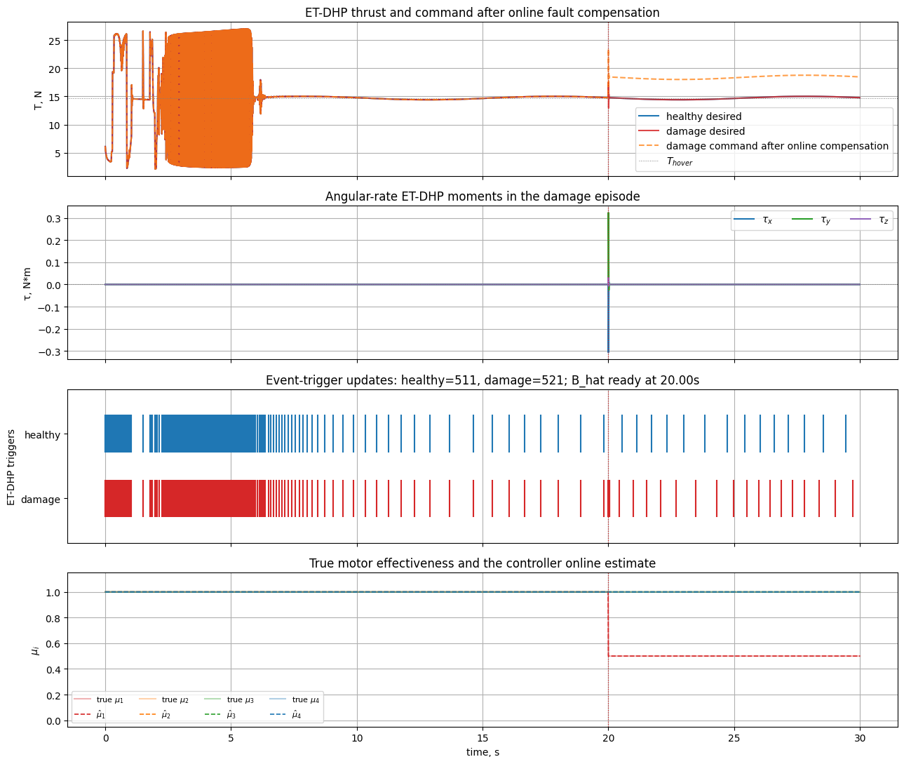
Sine altitude tracking with an ET-DHP controller that updates its plant-network online. At t = 20 s the M1 = 50% fault triggers, the plant-network adapts its \(\hat\mu\) estimate over a few event-trigger updates, and the controller compensates the asymmetry with an elevated thrust command:

Detailed 4-panel breakdown — thrust, moments, event-trigger ticks and motor-effectiveness estimate:

1. Built-in preset: 50% motor loss (Lu 2019)¶

The simplest way to reproduce a canonical FTC scenario — import a ready-made profile and pass it to the env via damage_profile.

import gymnasium as gym
import numpy as np

import tensoraerospace
from tensoraerospace.aerospacemodel.quadrotor.damage import LU_M1_50PCT_LOSS

env = gym.make(
    "NonlinearQuadrotor-v0",
    initial_state=np.zeros(12),
    number_time_steps=1000,
    damage_profile=LU_M1_50PCT_LOSS,
)

obs, _ = env.reset()
T_hover = env.unwrapped.model.hover_thrust
for k in range(1000):
    obs, _, _, trunc, info = env.step(np.array([T_hover, 0.0, 0.0, 0.0]))
    if "damage_events_triggered" in info:
        print(f"t = {k*0.01:.2f} s — fired: {info['damage_events_triggered']}")
        print(f"  motor μ: {info['damage_state']['mu']}")
    if trunc:
        break

2. Custom event: M2 loses 70% effectiveness at t=3 s¶

Build your own DamageProfile from any combination of events.

from tensoraerospace.aerospacemodel.quadrotor.damage import (
    DamageProfile, RotorDamageEvent,
)

profile = DamageProfile(events=[
    RotorDamageEvent(trigger_time=3.0, rotor_id=1, mu=0.3, label="m2_70pct_loss"),
])

3. Multiple full losses staggered in time¶

from tensoraerospace.aerospacemodel.quadrotor.damage import (
    DamageProfile, RotorLossEvent,
)

profile = DamageProfile(events=[
    RotorLossEvent(trigger_time=2.0, rotor_id=0, label="m1_lost"),
    RotorLossEvent(trigger_time=4.0, rotor_id=2, label="m3_lost"),  # uncontrollable
])

RotorLossEvent is shorthand for mu = 0. After t = 4 s only two rotors (M2 and M4) remain — physically equivalent to total loss of controllability in an X-frame.

4. Gradual wear: exponential decay of μ¶

The wear model μ̇ = −(1/τ)(μ − μ_floor) arms at trigger_time and exponentially drives the rotor effectiveness to mu_floor. Useful for long-endurance simulations.

from tensoraerospace.aerospacemodel.quadrotor.damage import (
    DamageProfile, MotorEfficiencyDecay,
)

# Motor 3 degrades with 8 s time constant down to 30% effectiveness
wear = DamageProfile(events=[
    MotorEfficiencyDecay(
        trigger_time=2.0,
        rotor_id=2,
        tau=8.0,
        mu_floor=0.3,
        label="m3_wear",
    ),
])

After t ≈ 3·τ ≈ 24 s μ reaches ~mu_floor + 0.05·(1 - mu_floor).

5. Runtime injection (single-fire)¶

You can also inject events at runtime — for instance, in response to an anomaly detector. Each injected event fires once and is cleared by env.reset().

import numpy as np

from tensoraerospace.aerospacemodel.quadrotor.damage import RotorLossEvent
from tensoraerospace.envs.quadrotor import NonlinearQuadrotorEnv

env = NonlinearQuadrotorEnv(
    initial_state=np.zeros(12),
    number_time_steps=1000,
    action_space="virtual",
    damage_profile=None,
)
env.reset()
T_hover = env.model.hover_thrust

for k in range(1000):
    if k == 300:  # surprise — M4 lost at t = 3 s
        env.damage_manager.inject_event(
            RotorLossEvent(trigger_time=3.0, rotor_id=3, label="emergency_m4_loss")
        )
    obs, _, _, trunc, info = env.step(np.array([T_hover, 0.0, 0.0, 0.0]))

6. Logging events via callback¶

Pass damage_event_callback=f(event, state) to receive an explicit notification every time an event fires. Convenient for TensorBoard / Weights & Biases hooks.

import numpy as np

from tensoraerospace.aerospacemodel.quadrotor.damage import LANZON_M1_LOSS
from tensoraerospace.envs.quadrotor import NonlinearQuadrotorEnv

events_log = []

def on_damage(event, state):
    events_log.append({
        "label": event.label,
        "rotor": event.rotor_id,
        "mu_after": float(state.mu[event.rotor_id]),
        "all_mu": state.mu.copy(),
    })

env = NonlinearQuadrotorEnv(
    initial_state=np.zeros(12),
    number_time_steps=1000,
    action_space="virtual",
    damage_profile=LANZON_M1_LOSS,
    damage_event_callback=on_damage,
)
env.reset()
# ...run episode...
print(events_log)

7. Reading damage state from info-dict¶

After every env.step(...), info contains a snapshot of all 4 motors’ effectiveness and the effective/commanded ω² (when a damage manager is active).

import numpy as np

from tensoraerospace.aerospacemodel.quadrotor.damage import WEAR_DEGRADATION_M3
from tensoraerospace.envs.quadrotor import NonlinearQuadrotorEnv

env = NonlinearQuadrotorEnv(
    initial_state=np.zeros(12),
    number_time_steps=2500,
    action_space="virtual",
    damage_profile=WEAR_DEGRADATION_M3,
)
obs, _ = env.reset()
T_hover = env.model.hover_thrust
mu_history = []
for k in range(2500):
    obs, _, _, trunc, info = env.step(np.array([T_hover, 0.0, 0.0, 0.0]))
    mu_history.append(info["damage_state"]["mu"].copy())
    if trunc:
        break

mu_arr = np.array(mu_history)
print(f"Final μ: {mu_arr[-1]}")
# μ_3 → 0.30, others = 1.0

8. Damage in `rotor` action_space mode¶

If your controller emits rotor-level commands [ω₁², ω₂², ω₃², ω₄²], switch to action_space="rotor". The env will apply μ to the command before re-mixing into (T, τ) for the integrator.

import gymnasium as gym
import numpy as np

import tensoraerospace
from tensoraerospace.aerospacemodel.quadrotor.damage import LU_M1_50PCT_LOSS

env = gym.make(
    "NonlinearQuadrotor-v0",
    initial_state=np.zeros(12),
    number_time_steps=500,
    action_space="rotor",
    damage_profile=LU_M1_50PCT_LOSS,
)
obs, _ = env.reset()
# In hover all four rotors carry the same ω² = T_hover / (4·k_T)
T_hover = 1.5 * 9.81
omega2_hover = T_hover / (4 * env.unwrapped.allocator.k_T)
action = np.full(4, omega2_hover)

for k in range(500):
    obs, _, _, trunc, info = env.step(action)

9. Reset and replay¶

env.reset() zeroes all μ and clears injected events but keeps the profile. Run multiple episodes with the same fault injection.

import numpy as np

from tensoraerospace.aerospacemodel.quadrotor.damage import LANZON_M1_LOSS
from tensoraerospace.envs.quadrotor import NonlinearQuadrotorEnv

env = NonlinearQuadrotorEnv(
    initial_state=np.zeros(12),
    number_time_steps=1000,
    action_space="virtual",
    damage_profile=LANZON_M1_LOSS,
)

for episode in range(3):
    env.reset()
    print(f"Episode {episode}: μ at start = {env.damage_manager.state.mu}")

10. Switching profile via `reset(options=...)`¶

You can swap the profile without re-creating the env — handy for multi-task curricula where each episode carries a different fault scenario.

import numpy as np

from tensoraerospace.aerospacemodel.quadrotor.damage import (
    LANZON_M1_LOSS, LU_M1_50PCT_LOSS, WEAR_DEGRADATION_M3,
)
from tensoraerospace.envs.quadrotor import NonlinearQuadrotorEnv

env = NonlinearQuadrotorEnv(
    initial_state=np.zeros(12),
    number_time_steps=1000,
    action_space="virtual",
)

scenarios = [LANZON_M1_LOSS, LU_M1_50PCT_LOSS, WEAR_DEGRADATION_M3]
for sc in scenarios:
    env.reset(options={"damage_profile": sc})
    # ...run one episode under this scenario...