Building the Simulink Model
In this lesson we transfer the state-space matrices \(A\), \(B\), \(C\), \(D\) from the MATLAB script (see Lesson 4) into a Simulink diagram, get a working dynamic model, and prepare it for code generation into a DLL/SO that can be called from Python (see Lesson 6).
Why move the model into Simulink
A MATLAB script is convenient for computation but is not a real-time simulator. Simulink adds several features the bare script does not have:
- Discrete time integrators (fixed or variable step) with automatic synchronisation of every block.
- Graphical interface that exposes the structure of the control object as a block diagram — useful for debugging and for documentation.
- Embedded Coder code generation turns the model into C/C++ with a
fixed
dt, ready to be embedded in a DLL/SO and called from Python viactypes. Without this step the Python wrapper in Lesson 6 cannot be built.
Creating the control system in Simulink
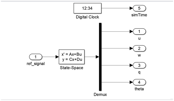
To create the control system in Simulink, follow these steps:
- Add components from the Simulink library to the canvas:
- Simulink/Continuous/State-Space — implements the equations \(\dot{x} = Ax + Bu\), \(y = Cx + Du\) in a single block. This is your control system.
- Simulink/Sources/Digital Clock — provides simulation time; useful for logging and for blocks that explicitly depend on \(t\).
- Simulink/Commonly Used Blocks/In1 — external model input
(control vector \(u\)). Embedded Coder turns it into a field of the
ExtUstruct during code generation. - Simulink/Commonly Used Blocks/Out1 — external model output
(vector \(y\)). It becomes a field of
ExtYafter code generation. - Rename the In1/Out1 blocks to meaningful signal names — for
example
ref_signalfor the input,u/w/q/thetafor the output components. These names propagate one-to-one into the C structs and into thectypeswrapper on the Python side (Lesson 6). - Specify the State-Space block parameters — most conveniently as references to MATLAB workspace variables:
- A: name of the state matrix (filled from the Lesson 4 script).
- B: control matrix.
- C, D: observation and feedthrough matrices. If all state components are exposed as outputs, typically \(C = I\) and \(D = 0\).
- Initial conditions: initial state vector \(x_0\) (often
zeros).
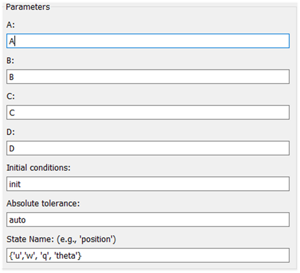
Solver configuration
Before running, open Simulation → Model Configuration Parameters and set:
- Solver type:
Fixed-step(required for code generation — Embedded Coder does not support variable-step solvers). - Fixed-step size: the same
dtyou use in your Python env (e.g.0.01s for the F-16,0.02s for the B747). - Stop time: simulation duration; only affects standalone Simulink runs, in code generation it is driven by the external loop.
- Solver:
ode4 (Runge-Kutta)— a good trade-off between accuracy and predictability for linear and weakly nonlinear systems.
Match dt everywhere
If dt differs between Simulink and your Python wrapper (Lesson 6),
the dynamics are distorted: the discretised matrices \(A_d, B_d\)
depend on dt. Best practice is to define dt once as a constant in
the MATLAB script and reference it both in the Simulink solver
settings and in the Python code.
Pre-codegen smoke test
Run the simulation from Simulink (Ctrl+T) with a test input — say, a
step from a Step block — and verify:
- The
Out1plots match a direct computation of \(y = Ce^{At}x_0 + \int_0^t Ce^{A(t-\tau)}Bu(\tau)\,d\tau\) in MATLAB. - No
Algebraic looporSample time mismatchwarnings. - Signal dimensions on the ports are consistent with the dimensions of
A,B,C,D.
After this you can move on to Lesson 6 — Embedded Coder codegen and DLL/SO build for Python.