Walkthrough: F-16 control with IHDP (step-by-step)¶

A clear step-by-step example based on example_ihdp_beautiful.ipynb: from creating the reference signal to running IHDP and interpreting the plots. FAQ and practical tips are at the end.

For the concise version of the same task, see Example: IHDP on the linear F-16. For the harder sinusoidal-tracking setup on the nonlinear plant, see Example: IHDP on the nonlinear F-16.

-- Step 1. Simulation time and reference signal

-- Step 2. F-16 environment

-- Step 3. IHDP parameters

-- Step 4. Create the agent

-- Step 5. Simulation

-- Step 6. Plots and expectations

-- FAQ and tips

Step 1. Simulation time and reference signal¶

Define the discretization and modeling horizon. Form a step reference signal for the angle of attack alpha: this is the target the agent will try to reach by minimizing the tracking error.

import numpy as np
from tensoraerospace.utils import generate_time_period, convert_tp_to_sec_tp
from tensoraerospace.signals.standard import unit_step

dt = 0.01  # discretization step, s
tp = generate_time_period(tn=20, dt=dt)  # array of time steps
tps = convert_tp_to_sec_tp(tp, dt=dt)    # time in seconds for plots
number_time_steps = len(tp)

# Step reference for angle of attack (5 deg) at the 10th step
reference_signals = unit_step(degree=5, tp=tp, time_step=10, output_rad=True).reshape(1, -1)

Step 2. Initialize the F-16 environment¶

Create the LinearLongitudinalF16-v0 environment. Specify the initial state, the composition of the state/output vectors, and the control channel (elevator -- ele). Enable tracking_states=["alpha"] to orient the training toward tracking the angle of attack.

import gymnasium as gym

env = gym.make(
    'LinearLongitudinalF16-v0',
    number_time_steps=number_time_steps,
    initial_state=[[0], [0], [0]],   # order: [theta, alpha, q]
    reference_signal=reference_signals,
    use_reward=False,
    state_space=["theta", "alpha", "q"],
    output_space=["theta", "alpha", "q"],
    control_space=["ele"],
    tracking_states=["alpha"],
)

obs, info = env.reset()

Step 3. Actor / Critic / Incremental model parameters¶

IHDP uses three modules:

Actor -- a neural network that outputs the control action based on the tracking error.
Critic -- a neural network that estimates the cost functional J(x) and its gradient.
Incremental model -- online identification and local linearization of the dynamics.

The parameters below are tuned for the demonstration case: a strong persistent excitation component (type_PE="combined") speeds up the identification; high learning_rate values are appropriate for a short horizon and saturation limits (WB_limits).

actor_settings = {
    "start_training": 5,
    "layers": (25, 1),
    "activations": ("tanh", "tanh"),
    "learning_rate": 2.0,
    "learning_rate_exponent_limit": 10,
    "type_PE": "combined",
    "amplitude_3211": 15,
    "pulse_length_3211": 5 / dt,
    "maximum_input": 25,
    "maximum_q_rate": 20,
    "WB_limits": 30,
    "NN_initial": 120,
    "cascade_actor": False,
    "learning_rate_cascaded": 1.2,
}

critic_settings = {
    "Q_weights": [8],
    "start_training": -1,
    "gamma": 0.99,
    "learning_rate": 15.0,
    "learning_rate_exponent_limit": 10,
    "layers": (25, 1),
    "activations": ("tanh", "linear"),
    "WB_limits": 30,
    "NN_initial": 120,
    "indices_tracking_states": env.unwrapped.indices_tracking_states,
}

incremental_settings = {
    "number_time_steps": number_time_steps,
    "dt": dt,
    "input_magnitude_limits": 25,
    "input_rate_limits": 60,
}

Step 4. Create the IHDP agent¶

Pass the module configurations and environment metadata to the agent. Make sure that indices_tracking_states is consistent with the ordering of the environment states.

from tensoraerospace.agent.ihdp.model import IHDPAgent

agent = IHDPAgent(
    actor_settings,
    critic_settings,
    incremental_settings,
    env.unwrapped.tracking_states,
    env.unwrapped.state_space,
    env.unwrapped.control_space,
    number_time_steps,
    env.unwrapped.indices_tracking_states,
)

Step 5. Main simulation loop¶

At each step:

agent.predict returns the control action given the current state and reference signal,
the environment integrates the dynamics and returns the new state,
if needed, you can use reward (here it is disabled for pure tracking control).

from tqdm import tqdm

xt = np.array([[0], [0], [0]])  # initial state [theta, alpha, q]
for step in tqdm(range(number_time_steps - 3)):
    ut = agent.predict(xt, reference_signals, step)
    xt, reward, terminated, truncated, info = env.step(np.array(ut))
    if terminated or truncated:
        break

Step 6. Visualize results¶

Compare the alpha trajectory with the reference signal and analyze the wz dynamics. Smoothness and absence of overshoot depend on the critic weights, constraints, and learning rates.

env.unwrapped.model.plot_transient_process('alpha', tps, reference_signals[0], to_deg=True, figsize=(15, 4))

env.unwrapped.model.plot_state('wz', tps, to_deg=True, figsize=(15, 4))

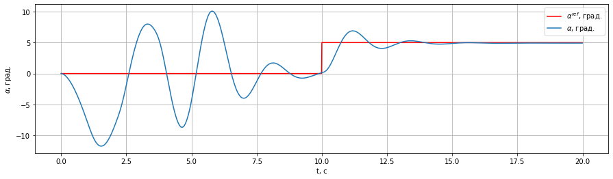
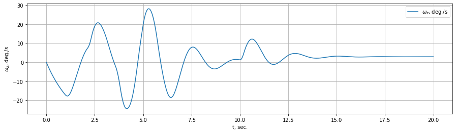
Expected signs of correct operation:

The alpha error quickly converges to zero without sustained oscillations
wz stays within physically reasonable bounds and decays
The control signal (if plotted) does not saturate for extended periods

Note

The training parameters are tuned for demonstration purposes and may differ from the optimal ones for your task.

Sanity checks¶

The mean absolute error of alpha over the final 20% of the horizon is less than 5-10% of the step amplitude
No prolonged saturation of the control signal
The discrete step dt is consistent with the dynamics (no "sawtooth" noise)

Units and normalization¶

Angles theta, alpha, q in the models and plots are in radians; for visualization they are converted to degrees (to_deg=True)
The control ele is in radians; limits are specified in the same units
If you use custom features, normalize inputs for stable training

Frequently asked questions and tips¶

Why is persistent excitation (PE) added? For quality identification of the incremental model, the input must have rich dynamics; otherwise the actor and critic quickly "get stuck."
How to choose the critic's Q_weights? Increasing the weight on the tracking error (e.g., on alpha) raises the priority of tracking accuracy relative to control effort.
What to do about control chattering? Reduce the learning_rate, increase WB_limits carefully, limit maximum_input/maximum_q_rate, and check feature scaling.
How to speed up convergence? Increase the actor/critic learning_rate, but monitor stability; increase the PE amplitude if identification is slow.