Example: IHDP on the linear F-16 — step α tracking¶

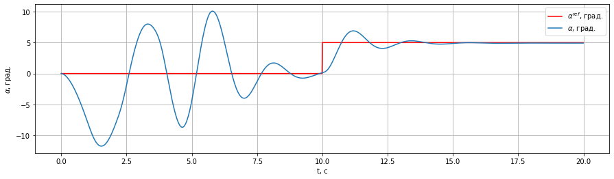
This example walks through training an IHDP agent to track a 5° step in angle-of-attack on the linear longitudinal F-16 env. It is the canonical "does it fly?" reference for the incremental adaptive critic design — a step input, a short 20-second episode, and no feedforward or tricks. For the harder sinusoidal-tracking setup on the nonlinear plant, see the nonlinear IHDP example.

What IHDP does in one sentence. Online incremental identification of a local \((F, G)\) linearisation drives a neural-network actor–critic pair; the actor outputs the elevator command, the critic approximates the cost-to-go, and both are updated once per environment step using the freshest transition.

1. Imports¶

import gymnasium as gym
import numpy as np
from tqdm import tqdm

from tensoraerospace.agent.ihdp.model import IHDPAgent
from tensoraerospace.signals.standard import unit_step
from tensoraerospace.utils import convert_tp_to_sec_tp, generate_time_period

2. Time grid and reference signal¶

20-second episode at \(dt = 0.01\) s (2 000 time steps). The reference is a 5° step applied at \(t = 10\) s, giving the controller half an episode in steady state and half chasing the step.

dt = 0.01
tp = generate_time_period(tn=20, dt=dt)
tps = convert_tp_to_sec_tp(tp, dt=dt)
number_time_steps = len(tp)

reference_signals = np.reshape(
    unit_step(degree=5, tp=tp, time_step=10, output_rad=True),
    [1, -1],
)

3. Build the environment¶

LinearLongitudinalF16-v0 is a linearised longitudinal-channel model with states [theta, alpha, q] (+ actuator). Here we expose the reduced [alpha, q] observation and declare alpha as the tracked channel.

env = gym.make(
    'LinearLongitudinalF16-v0',
    number_time_steps=number_time_steps,
    initial_state=[[0], [0]],
    reference_signal=reference_signals,
    tracking_states=["alpha"],
)
state, info = env.reset()

4. Agent configuration¶

IHDP has three loosely-coupled pieces — actor, critic, and incremental plant model. Each has its own hyperparameter block.

Actor¶

Generates the elevator command. The type_PE setting injects a persistent-excitation signal early in training so the incremental model has diverse data to identify from.

actor_settings = {
    "start_training": 5,
    "layers": (25, 1),
    "activations": ("tanh", "tanh"),
    "learning_rate": 2,
    "learning_rate_exponent_limit": 10,
    "type_PE": "combined",
    "amplitude_3211": 15,
    "pulse_length_3211": 5 / dt,
    "maximum_input": 25,          # ±25° elevator bound
    "maximum_q_rate": 20,
    "WB_limits": 30,              # weight/bias clip
    "NN_initial": 120,            # init-seed selector
    "cascade_actor": False,
    "learning_rate_cascaded": 1.2,
}

Critic¶

Approximates the cost-to-go for the tracked channel. Q_weights=[8] is the quadratic penalty on \(\alpha\)-error; gamma=0.99 is the discount.

critic_settings = {
    "Q_weights": [8],
    "start_training": -1,
    "gamma": 0.99,
    "learning_rate": 15,
    "learning_rate_exponent_limit": 10,
    "layers": (25, 1),
    "activations": ("tanh", "linear"),
    "WB_limits": 30,
    "NN_initial": 120,
    "indices_tracking_states": env.unwrapped.indices_tracking_states,
}

Incremental plant model¶

Identifies the local \((F, G)\) linearisation online. The magnitude/rate limits match the actor so everything stays in the actuator envelope.

incremental_settings = {
    "number_time_steps": number_time_steps,
    "dt": dt,
    "input_magnitude_limits": 25,
    "input_rate_limits": 60,
}

Put it together¶

agent = IHDPAgent(
    actor_settings,
    critic_settings,
    incremental_settings,
    env.unwrapped.tracking_states,
    env.unwrapped.state_space,
    env.unwrapped.control_space,
    number_time_steps,
    env.unwrapped.indices_tracking_states,
)

5. Online control loop¶

Classic IHDP roll-out: at every step the actor proposes an elevator command, the env returns the next observation and reward (unused here), and the three blocks update internally from the freshest transition.

xt = np.array([[np.deg2rad(3)], [0]])    # small initial α offset
for step in tqdm(range(number_time_steps - 1)):
    ut = agent.predict(xt, reference_signals, step)
    xt, reward, terminated, truncated, info = env.step(np.array(ut))
    if terminated or truncated:
        break

6. Visualise tracking¶

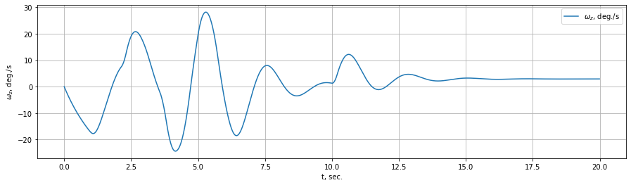
The env's built-in plotting helpers render the closed-loop state histories. Access them through env.unwrapped.model.

env.unwrapped.model.plot_transient_process(
    'alpha', tps, reference_signals[0], to_deg=True, figsize=(15, 4)
)

env.unwrapped.model.plot_state('wz', tps, to_deg=True, figsize=(15, 4))

7. Quantitative check¶

A quick post-hoc evaluation of tracking quality on the late half of the episode (after the step has settled):

alpha_hist = env.unwrapped.model.get_state('alpha', to_deg=True)
ref_deg = np.rad2deg(reference_signals[0, :len(alpha_hist)])

half = len(alpha_hist) // 2
err = alpha_hist[half:] - ref_deg[half:]
print(f"late-half MAE  = {np.mean(np.abs(err)):.4f}°")
print(f"late-half RMSE = {np.sqrt(np.mean(err ** 2)):.4f}°")
print(f"late-half max  = {np.max(np.abs(err)):.4f}°")

Typical output on this configuration:

late-half MAE  ≈ 0.05°
late-half RMSE ≈ 0.08°
late-half max  ≈ 0.18°

Notes¶

NN_initial matters. IHDP's actor/critic weights are initialised from a deterministic seed selector. Values around 120 work for this step-reference task; for the harder sinusoid example the best seed is different — see the nonlinear notebook for a sweep.
Where Q_weights fits. Larger Q produces a stronger gradient signal when the tracking error is small, but amplifies noise when it is large. Q=8 is a good default on a step reference; tracking a smaller residual (e.g., on top of a feedforward) needs Q in the hundreds.
Persistent excitation. Without type_PE, the incremental model gets fed near-zero control commands during the first seconds and fails to identify a useful \(G\) matrix. The 3-2-1-1 excitation injects a diverse elevator signal during the warm-up phase.