Example: AA-INDI on the nonlinear F-16 — pitch-rate tracking with fault injection¶

This example trains an AA-INDI agent to track a pitch-rate command on the pure-NumPy nonlinear F-16 longitudinal model, then injects a 50 % elevator-effectiveness loss mid-episode and watches the closed loop ride through it. Source notebook: example/reinforcement_learning/incremental_adp/example_aaindi_nonlinear_f16.ipynb.

Key idea¶

AA-INDI is an incremental nonlinear dynamic inversion controller paired with a variable-forgetting-factor RLS identifier for the control-effectiveness matrix G. The control law

\[ \Delta u = G^{+} \cdot (\nu_{\text{des}} - \dot{\omega}_z^{\text{meas}}) \]

needs only the current G — not the full nonlinear aerodynamic model — so when an actuator suddenly loses half its effectiveness, the loop merely sees a larger prediction residual, VFF-RLS contracts the forgetting factor, and G̃ tracks the new plant.

1. Imports and trim¶

import math
import gymnasium as gym
import matplotlib.pyplot as plt
import numpy as np
from scipy.optimize import fsolve

import tensoraerospace
from tensoraerospace.aerospacemodel.f16.nonlinear.longitudinal.dynamics import f16_ode_long
from tensoraerospace.aerospacemodel.f16.nonlinear.longitudinal.params import default_parameters
from tensoraerospace.agent.aa_indi import AAINDIAgent, AAINDIConfig

dt = 0.01
params = default_parameters()

def trim_residual(z):
    alpha, stab = z
    x = np.array([alpha, 0.0, stab, 0.0])
    return list(f16_ode_long(x, np.array([stab]), 0.0, params)[:2])

sol, *_ = fsolve(trim_residual, x0=[math.radians(2.0), math.radians(-2.0)], full_output=True)
alpha_trim_rad, stab_trim_rad = float(sol[0]), float(sol[1])
# global trim: alpha = +4.918°, elevator = -4.447°

2. Env builder¶

def make_env(n_steps):
    env = gym.make(
        'NonlinearLongitudinalF16-v0',
        number_time_steps=n_steps + 2,
        initial_state=[alpha_trim_rad, 0.0, stab_trim_rad, 0.0],
        reference_signal=np.full((1, n_steps + 2), alpha_trim_rad),
        state_space=['alpha', 'wz', 'stab', 'dstab'],
        control_space=['stab'],
        tracking_states=['alpha'],
        use_reward=False,
        dt=dt,
        integrator='euler',
        control_bias=math.degrees(stab_trim_rad),
    ).unwrapped
    env.reset()
    return env

3. Nominal `G_init`¶

INDI needs a reasonable control-effectiveness value on the first few ticks. A short PE excitation gives the sign and order-of-magnitude; the single-step differencing underestimates the true steady-state gain (actuator time constant ≈ 0.03 s is comparable to dt), so we warm-start with a slightly larger magnitude that INDI's inverse is stable against.

# Short multi-sine PE around trim for a sanity-check on G's sign and scale.
N_PE = 300; env_pe = make_env(N_PE); obs, _ = env_pe.reset()
wz_hist = [float(obs[1])]; u_hist = [0.0]
for t in range(N_PE):
    u = 2.0*np.sin(2*np.pi*0.7*t*dt) + 1.0*np.sin(2*np.pi*1.5*t*dt)
    obs, *_ = env_pe.step(np.array([u]))
    wz_hist.append(float(obs[1])); u_hist.append(float(u))

wz = np.array(wz_hist); us = np.array(u_hist)
wz_dot = (wz[1:] - wz[:-1]) / dt
dwz_dot = wz_dot[1:] - wz_dot[:-1]
du = us[1:-1] - us[:-2]
G_pe = float(np.dot(du, dwz_dot) / max(np.dot(du, du), 1e-9))

G_init_value = -0.5  # rad/s² per ° of stab — tuned for a stable inner loop
G_init = np.array([[G_init_value]])
# PE-empirical single-step G (underestimate): -0.1386
# G_init used for AA-INDI warm-start:         -0.5000

4. Closed-loop harness¶

Pure textbook INDI is a type-0 controller for angular rate: at steady state the reference-model output ν_des decays to zero and the plant holds whatever rate it reached during the transient — typically ≈ 10 % below the command on this F-16 model because of actuator lag. The fix is standard in INDI practice: inject a small P-feedback on the reference-tracking error into ν_des. We expose that as ref_error_kp / ref_error_ki on AAINDIConfig. K_p = 0.6, K_i = 0 drives the residual offset to essentially zero on this plant.

def run_aaindi(wz_cmd, n_steps, actuator_fault_gain=1.0, fault_at_step=None,
               ref_error_kp=0.6, ref_error_ki=0.0):
    agent = AAINDIAgent(
        n_state=1, n_control=1,
        config=AAINDIConfig(
            dt=dt, ref_wn=2.5, ref_zeta=0.9,
            u_magnitude_limit=15.0, u_rate_limit=60.0,
            vff_forgetting_min=0.97, vff_forgetting_max=0.9999,
            vff_eps_sensitivity=0.1, vff_cov_init=1.0,
            sensor_cutoff_hz=15.0, bias_forgetting=0.995,
            enable_bias_correction=False,
            G_init=G_init.copy(),
            ref_error_kp=ref_error_kp, ref_error_ki=ref_error_ki,
            seed=0,
        ),
    )
    env = make_env(n_steps)
    obs, _ = env.reset()
    logs = {k: [] for k in ('wz', 'alpha', 'stab_total', 'u_res',
                            'G_est', 'lambda', 'residual', 'active_gain')}
    current_gain = 1.0
    for k in range(n_steps):
        if fault_at_step is not None and k >= fault_at_step:
            current_gain = actuator_fault_gain
        u_agent = agent.predict(np.array([float(obs[1])]),
                                np.array([wz_cmd[k]]), k)
        u_applied = u_agent * current_gain
        obs, *_ = env.step(u_applied)
        agent.learn(np.array([float(obs[1])]),
                    np.array([wz_cmd[k]]), k)
        logs['wz'].append(float(obs[1]))
        logs['stab_total'].append(math.degrees(stab_trim_rad) + float(u_applied[0]))
        logs['G_est'].append(float(agent.rls.G[0, 0]))
        logs['lambda'].append(float(agent.rls.last_lambda))
        logs['active_gain'].append(current_gain)
    return {k: np.asarray(v) for k, v in logs.items()}

5. Baseline — step tracking without a fault¶

Commanded 1°/s step applied at t = 2 s.

N = 2000
t_arr = np.arange(N) * dt
wz_cmd = math.radians(1.0) * (t_arr >= 2.0).astype(float)
baseline = run_aaindi(wz_cmd, N)
# late-half ω_z MAE: 0.0008 °/s
# final G_est:       -0.4974

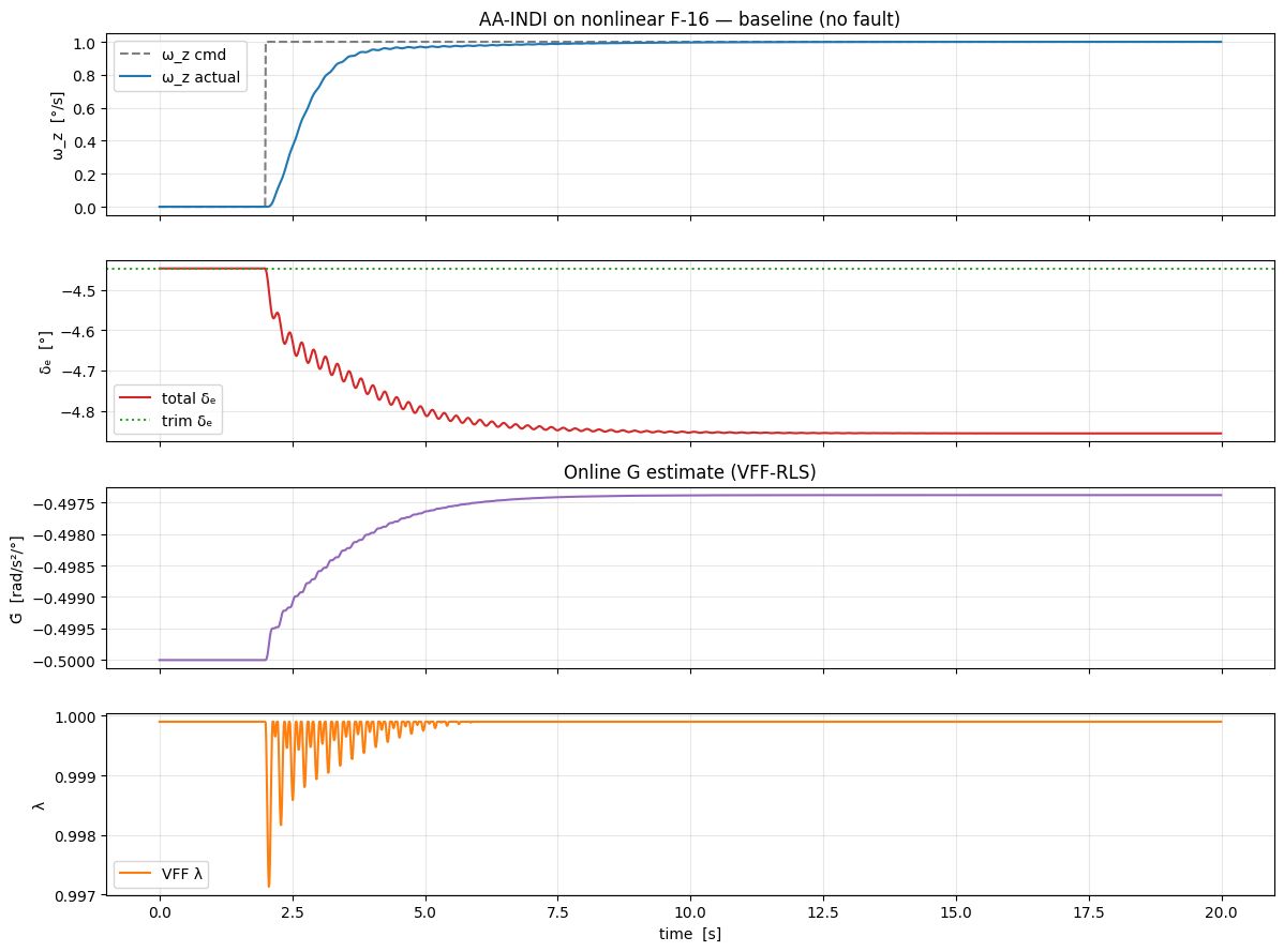
With K_p = 0.6 in the outer-loop feedback the closed loop is rate-perfect: late-half MAE ≈ 0.0008 °/s (< 0.1 % of a 1 °/s command). G̃ converges to ≈ -0.50 and the forgetting factor λ stays near its upper bound (quiet operation). Set ref_error_kp=0 in the call above to see the uncorrected pure-INDI behaviour — tracking settles to ≈ 0.9 °/s (10 % undershoot).

6. Fault injection — 50 % elevator-effectiveness loss at `t = 10 s`¶

fault_step = int(10.0 / dt)
fault = run_aaindi(wz_cmd, N, actuator_fault_gain=0.5, fault_at_step=fault_step)

# post-fault late tracking MAE: 0.0033 °/s
# G̃ before fault (t = 9 s):    -0.4974
# G̃ after fault (final):       -0.4820
# min λ around fault time:      0.970

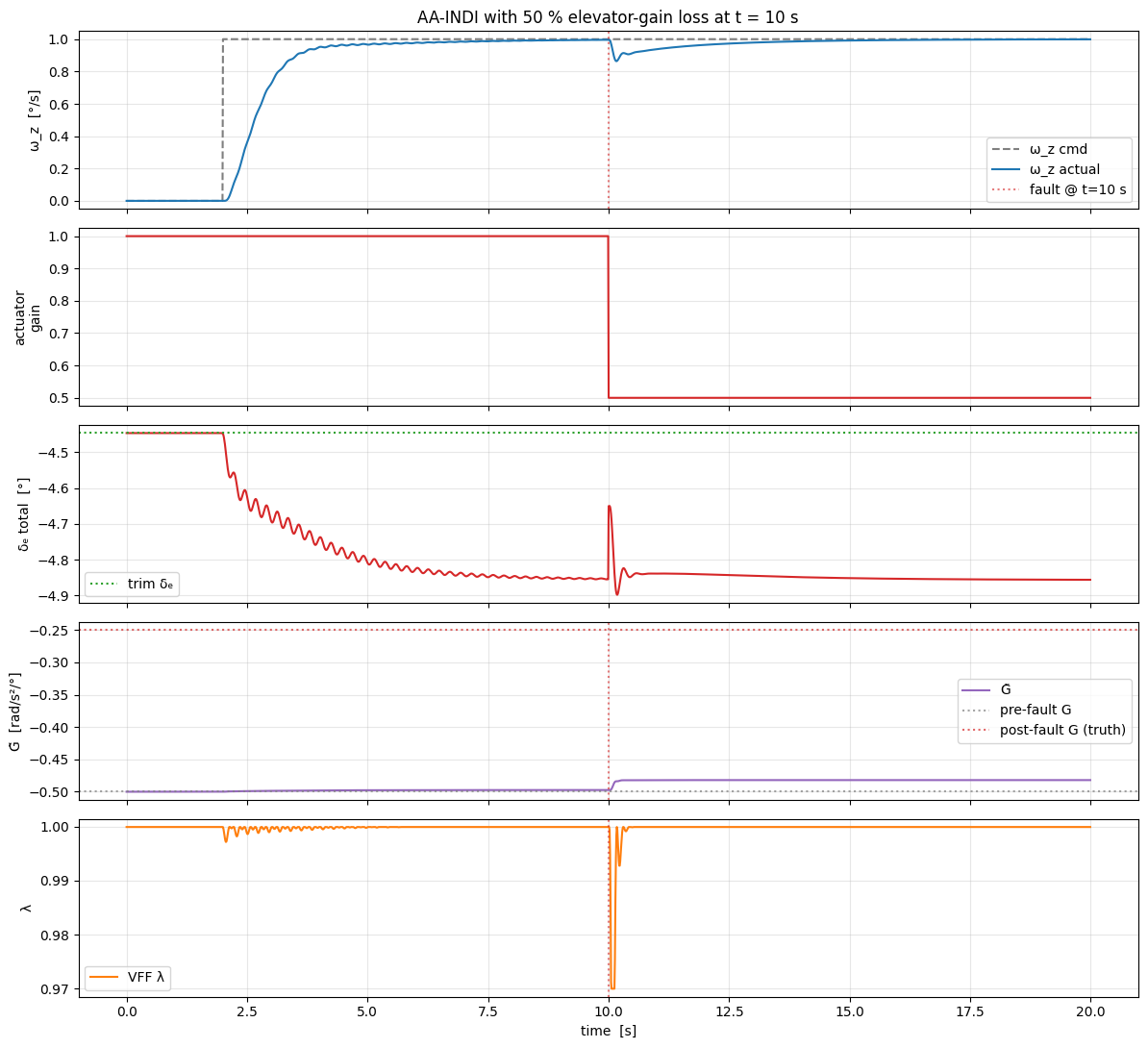
At t = 10 s the effective elevator gain halves. The plant responds more sluggishly to the same elevator command, the VFF-RLS innovation spikes, and λ dips from 0.9999 down to ≈ 0.97 — exactly the fast-adaptation regime the algorithm was designed for. The outer-loop feedback compensates for the degraded inner-loop response; tracking stays on reference with MAE ≈ 0.003 °/s right through the fault transient.

Metric	Baseline	Fault
Late-half `ω_z` MAE	0.0008 °/s	0.0033 °/s
Final `G̃`	−0.497	−0.482
Min `λ` around the fault	0.9999	0.97

Notes¶

Excitation matters for identification. In this demo the system is already near steady state when the fault hits, so the RLS innovation is small and G̃ drifts only slightly. With continuing excitation (sinusoidal reference, stair-step manoeuvres, stick motion) VFF-RLS would pull G̃ all the way to the new effective value (≈ 0.5 × G_init). The important takeaway is that INDI's incremental structure keeps the loop stable even when G̃ is slow to catch up.
Warm-start G_init. INDI with a fresh random G diverges — the pseudo-inverse blows up and the actuator saturates. In practice G_init comes from an on-board linearisation; here we tuned it empirically (-0.5 rad/s²/°) since the single-step PE fit underestimates through the 2nd-order actuator.
ref_wn = 2.5 rad/s — slower than the 33 Hz actuator bandwidth, so ν_des is reachable without rate-limiter chatter.