Lesson 8 — Introduction to Reinforcement Learning for Aerospace Control

1. Why Reinforcement Learning for Aerospace?

In Lessons 1--7 we studied classical control theory: state-space models, stability analysis, pole placement, observer design, and PID tuning. These methods have been the backbone of flight control for decades and remain indispensable. However, they come with well-known limitations:

• Fixed gains. A controller designed for one flight condition (altitude, speed, mass) may perform poorly at another. Gain scheduling partially addresses this but requires a large number of design points.
• Need for an accurate model. Pole placement and LQR rely on precise knowledge of the matrices \(A\), \(B\), \(C\), \(D\). In practice, aerodynamic coefficients are uncertain and change with wear, damage, or icing.
• Poor adaptation. Classical controllers do not learn from experience. If the plant changes (e.g., partial actuator failure), the controller cannot adjust itself.
• Difficulty with nonlinearities. Linearization is valid only near the operating point. Large-envelope maneuvers, stall regions, and coupling effects are hard to capture.

Reinforcement Learning (RL) offers a fundamentally different paradigm: instead of deriving a control law from a mathematical model, the controller learns by interacting with the system (or its simulation). The key advantages are:

• No explicit model required. The agent discovers how the system behaves through trial and error.
• Handles nonlinearities naturally. Neural network policies can represent highly nonlinear mappings.
• Adapts over time. Online or continual learning allows the policy to adjust to changing dynamics.
• Multi-objective optimization. The reward function can encode complex goals (tracking + fuel economy + structural load limits).

Real-world aerospace RL applications are already being explored:

• Attitude control of agile UAVs under wind disturbances
• Powered descent guidance for reusable rockets (SpaceX-style landing)
• Satellite station-keeping with limited propellant
• Adaptive flight control for damaged aircraft
• Autonomous air combat maneuvering

In this lesson we introduce the RL framework, relate it to the classical concepts you already know, and show how TensorAeroSpace brings both worlds together.

---

2. RL Fundamentals in 5 Minutes

2.1 Core Concepts

An RL system consists of two entities:

Concept	Classical Control Analogy	RL Term
Plant / Aircraft	Environment	Environment
Controller / Autopilot	Agent	Agent
Sensor readings	Observation / measurement	State \(s_t\)
Control input	Actuator command	Action \(a_t\)
Performance index	Cost function (LQR)	Reward \(r_t\)
Control law \(u = -Kx\)	Policy	Policy \(\pi(a \mid s)\)

At every discrete time step \(t\), the agent observes the state \(s_t\), selects an action \(a_t\) according to its policy \(\pi\), and the environment transitions to a new state \(s_{t+1}\) while returning a scalar reward \(r_t\). The goal of the agent is to maximize the expected cumulative reward:

\[J = \mathbb{E}\left[\sum_{t=0}^{T} \gamma^t r_t\right]\]

where \(\gamma \in [0,1]\) is the discount factor (how much the agent values future rewards relative to immediate ones).

2.2 Episode Structure

An episode is one complete interaction sequence:

reset() --> s_0
  |
  +--> agent selects a_0
  |       |
  |       +--> env.step(a_0) --> s_1, r_0, done_0
  |
  +--> agent selects a_1
  |       |
  |       +--> env.step(a_1) --> s_2, r_1, done_1
  |
  ... (repeat until done=True)

In aerospace terms: the episode starts at an initial flight condition, the autopilot issues elevator/throttle commands at each time step, and the episode ends when the simulation horizon is reached or the aircraft leaves the safe flight envelope.

2.3 Policy

The policy \(\pi\) is the mapping from observation to action. In classical control, the policy is an explicit formula such as \(u = -Kx\). In RL, it is typically a neural network:

\[a_t = \pi_\theta(s_t)\]

where \(\theta\) are the learnable parameters (weights) of the network. Training adjusts \(\theta\) to maximize \(J\).

Policies can be deterministic (\(a = \mu_\theta(s)\), used in DDPG) or stochastic (\(a \sim \pi_\theta(\cdot \mid s)\), used in PPO and SAC). Stochastic policies output a probability distribution over actions --- typically a Gaussian with learnable mean and standard deviation. This built-in randomness drives exploration: the agent tries slightly different control inputs and observes which ones yield higher rewards.

2.4 Value Functions and the Bellman Equation

Two value functions are central to RL:

• State-value function \(V^\pi(s)\) --- the expected cumulative reward starting from state \(s\) and following policy \(\pi\):

\[V^\pi(s) = \mathbb{E}_\pi\left[\sum_{k=0}^{\infty} \gamma^k r_{t+k} \;\middle|\; s_t = s\right]\]

• Action-value function \(Q^\pi(s,a)\) --- the expected cumulative reward starting from state \(s\), taking action \(a\), and then following policy \(\pi\):

\[Q^\pi(s,a) = \mathbb{E}_\pi\left[\sum_{k=0}^{\infty} \gamma^k r_{t+k} \;\middle|\; s_t = s, a_t = a\right]\]

Both satisfy the Bellman equation, which expresses a recursive relationship:

\[Q^\pi(s,a) = r(s,a) + \gamma \, \mathbb{E}_{s' \sim P}\left[V^\pi(s')\right]\]

In aerospace terms: \(Q^\pi(s,a)\) tells you "if the aircraft is in state \(s\) and I apply elevator deflection \(a\) right now, then follow my policy \(\pi\) afterwards, how well will the rest of the flight go?" The Bellman equation decomposes this into the immediate reward plus the discounted future value --- exactly the same structure as Bellman's principle of optimality in classical dynamic programming.

Actor-critic algorithms (A2C, PPO, SAC) maintain both a policy (actor) and a value function (critic). The critic evaluates how good the current policy is, and the actor improves the policy based on the critic's feedback.

2.5 On-Policy vs Off-Policy

RL algorithms fall into two broad categories:

• On-policy (PPO, A2C, A3C): The agent learns from data collected by its current policy. After each policy update, old data is discarded. Simple but data-hungry.
• Off-policy (SAC, DDPG, DQN, DSAC): The agent stores past experiences in a replay buffer and learns from them even after the policy has changed. More sample-efficient but can be less stable.

For aerospace applications where each simulation episode is expensive (high-fidelity CFD-coupled models, hardware-in-the-loop), off-policy algorithms like SAC are often preferred because they extract more learning from each interaction.

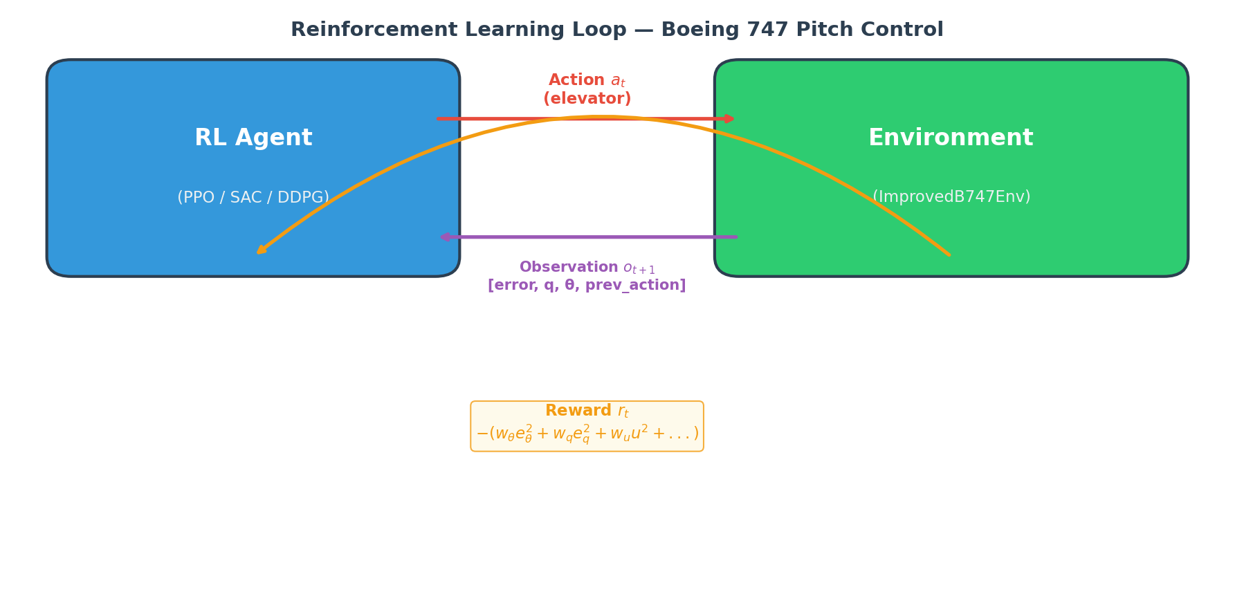
2.6 Agent-Environment Loop for B747 Pitch Tracking

Consider a Boeing 747 tracking a pitch angle reference. The diagram below shows one time step:

+------------------+         action: elevator         +---------------------+
|                  |     deflection  delta_e           |                     |
|   RL Agent       |  -------------------------------->|   B747 Environment  |
|   (Neural Net    |                                   |   (State-Space      |
|    Policy)       |<----------------------------------|    Model)           |
|                  |    state: [alpha, q, theta, ...]  |                     |
+------------------+    reward: -|theta - theta_ref|   +---------------------+

The state vector might include angle of attack \(\alpha\), pitch rate \(q\), pitch angle \(\theta\), and the tracking error. The reward penalizes deviation from the reference signal, encouraging the agent to learn a policy that tracks well.

---

3. RL vs Classical Control --- When to Use What

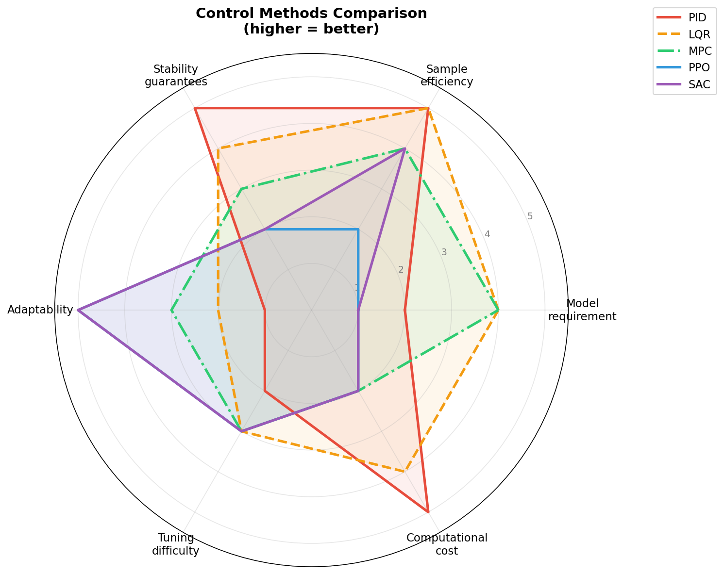
Criterion	PID	LQR / Pole Placement	MPC	RL (PPO/SAC)
Model requirement	None (tuned online)	Accurate linear model	Accurate model (can be nonlinear)	None (learns from data)
Adaptability	Low (fixed gains)	Low	Medium (re-solve online)	High (policy updates)
Computational cost (online)	Very low	Very low	High (optimization at each step)	Low (forward pass through NN)
Stability guarantees	Gain/phase margins	Lyapunov-based	Constraint satisfaction	No formal guarantees (empirical)
Handles constraints	No	Indirectly (weighting)	Yes (explicit)	Via reward shaping
Nonlinear systems	Linearize first	Linearize first	Directly	Directly
Ease of tuning	3 gains	Q, R matrices	Prediction horizon, cost	Reward function, hyperparameters
Multi-objective	Difficult	Weighting in Q, R	Multi-term cost	Flexible reward design

Rules of thumb:

• PID --- Use for simple SISO loops where you need a quick, reliable baseline with minimal compute (e.g., inner-loop rate damper).
• LQR / Pole Placement --- Use when you have a good linear model and want provable stability with optimal performance.
• MPC --- Use when you need to handle hard constraints (actuator limits, envelope protection) and have sufficient compute.
• RL --- Use when the system is complex, nonlinear, or uncertain; when you want the controller to adapt; or when the task involves multi-objective optimization that is hard to express analytically.

In practice, RL and classical methods are often combined: a classical controller provides a safe baseline, and RL fine-tunes or replaces it as it learns.

---

4. Key RL Algorithms in TensorAeroSpace

TensorAeroSpace ships with a variety of control algorithms --- both classical and learning-based. Here is a summary of each, with guidance on when to use it.

4.1 PPO --- Proximal Policy Optimization

from tensoraerospace.agent import PPO

• Type: On-policy, policy gradient
• Action space: Continuous
• Key idea: Clips the policy update to prevent destructively large steps, ensuring stable training.
• When to use: Your first choice for most aerospace RL tasks. Stable, general-purpose, works well with moderate amounts of data.

4.2 SAC --- Soft Actor-Critic

from tensoraerospace.agent import SAC

• Type: Off-policy, actor-critic with entropy regularization
• Action space: Continuous
• Key idea: Maximizes reward while also maximizing policy entropy, which encourages exploration and robustness.
• When to use: When you want better sample efficiency than PPO. Especially effective for continuous control with smooth dynamics.

4.3 DDPG --- Deep Deterministic Policy Gradient

from tensoraerospace.agent import DDPG

• Type: Off-policy, deterministic policy gradient
• Action space: Continuous
• Key idea: Learns a deterministic policy \(\mu(s)\) using a replay buffer and target networks.
• When to use: Single-action continuous control problems. Can be less stable than SAC; consider SAC first.

4.4 DSAC --- Distributional Soft Actor-Critic

from tensoraerospace.agent import DSAC

• Type: Off-policy, distributional RL
• Action space: Continuous
• Key idea: Models the full distribution of returns (not just the mean), enabling risk-aware control.
• When to use: When safety margins matter and you want to optimize worst-case performance (e.g., landing in crosswinds).

4.5 A2C --- Advantage Actor-Critic

from tensoraerospace.agent import A2C

• Type: On-policy, actor-critic
• Action space: Continuous or discrete
• Key idea: Synchronous variant of A3C. Uses advantage estimates to reduce variance.
• When to use: A simpler on-policy baseline. Good for educational purposes and quick experiments.

4.6 A3C --- Asynchronous Advantage Actor-Critic

from tensoraerospace.agent import Agent as A3CAgent

• Type: On-policy, asynchronous multi-worker
• Action space: Continuous or discrete
• Key idea: Runs multiple environment instances in parallel for faster exploration.
• When to use: When you have many CPU cores and want to speed up on-policy training.

4.7 DQN --- Deep Q-Network

from tensoraerospace.agent import DQNAgent

• Type: Off-policy, value-based
• Action space: Discrete only
• Key idea: Learns an action-value function \(Q(s,a)\) and acts greedily.
• When to use: Environments with discrete action spaces (e.g., Unity-based flight simulators with throttle levels).

4.8 GAIL --- Generative Adversarial Imitation Learning

from tensoraerospace.agent import GAIL

• Type: Imitation learning
• Action space: Continuous
• Key idea: Learns a policy by imitating expert demonstrations, using a discriminator to distinguish agent behavior from expert behavior.
• When to use: When you have recorded flight data from an expert pilot or an existing autopilot and want to clone that behavior.

4.9 ADP / ADHDP --- Adaptive Dynamic Programming

from tensoraerospace.agent import ADP
from tensoraerospace.agent import ADHDP

• Type: Neuro-dynamic programming
• Action space: Continuous
• Key idea: Approximates the Bellman equation using neural networks (action network + critic network). Rooted in optimal control theory.
• When to use: When you want an RL approach that is closely connected to classical dynamic programming and Bellman optimality.

4.10 HDP --- Heuristic Dynamic Programming

from tensoraerospace.agent import HDP

• Type: Neuro-dynamic programming
• Action space: Continuous
• Key idea: Model-based variant that uses a learned system model alongside actor-critic networks.
• When to use: When you have (or can learn) a forward model of the plant and want to exploit it for faster convergence.

4.11 IHDP --- Integral Heuristic Dynamic Programming

from tensoraerospace.agent import IHDPAgent

• Type: Neuro-dynamic programming (PyTorch-based)
• Action space: Continuous
• Key idea: Extends HDP with integral action for steady-state error elimination.
• When to use: Tracking problems where zero steady-state error is critical.

4.12 MPC --- Model Predictive Control

from tensoraerospace.agent import MPC

• Type: Model-based optimal control
• Action space: Continuous
• Key idea: Solves a finite-horizon optimization problem at each time step using a learned or known dynamics model.
• When to use: When you need constraint handling and have a good dynamics model. Bridges classical and learning-based control.

4.13 PID --- Classical PID Controller

While not an RL algorithm, TensorAeroSpace includes PID as a baseline controller. It is invaluable for comparison studies.

4.14 Algorithm Selection Flowchart

                    START
                      |
            Do you have expert data?
                   /        \
                 Yes          No
                  |            |
                GAIL     Is the action space discrete?
                          /            \
                        Yes              No
                         |                |
                        DQN      Do you need risk-awareness?
                                   /            \
                                 Yes              No
                                  |                |
                                DSAC      Do you need high sample efficiency?
                                            /            \
                                          Yes              No
                                           |                |
                                          SAC             PPO (start here)

---

5. The Gymnasium Interface

TensorAeroSpace environments follow the Gymnasium API. This means that every environment --- whether it models a B747, an F-16, a satellite, or a rocket --- exposes the same interface.

5.1 Key Methods

Method	Returns	Description
env.reset()	obs, info	Resets the environment to initial conditions. Returns the first observation and an info dictionary.
env.step(action)	obs, reward, terminated, truncated, info	Advances one time step. Returns the new observation, reward, termination flags, and info.

The two termination flags follow the Gymnasium convention:

• terminated --- The episode ended due to a physical condition (e.g., the aircraft stalled or the reference was perfectly tracked).
• truncated --- The episode ended because the time limit was reached.

The episode is done when terminated or truncated is True.

5.2 Observation and Action Spaces

For a typical longitudinal aircraft environment:

• Observation: A vector containing state variables (angle of attack, pitch rate, pitch angle, etc.) and possibly the tracking error and reference signal.
• Action: A vector of control surface deflections (e.g., elevator angle in radians).

Both spaces are continuous (gymnasium.spaces.Box).

5.3 Code Example: Running the B747 Environment

The following example creates an ImprovedB747Env, runs one episode with zero control input, and prints the total reward. This is the simplest way to interact with the environment.

import numpy as np
from tensoraerospace.envs import ImprovedB747Env
from tensoraerospace.signals.standard import unit_step
from tensoraerospace.utils import generate_time_period, convert_tp_to_sec_tp

# ----- Simulation parameters -----
dt = 0.1                                              # time step (seconds)
tp = generate_time_period(tn=40, dt=dt)               # time array
tps = convert_tp_to_sec_tp(tp, dt=dt)                 # time in seconds
number_time_steps = len(tp)                            # total steps

# Reference signal: 1-degree step in pitch angle (converted to radians)
reference = np.reshape(
    unit_step(degree=1, tp=tp, time_step=50, output_rad=True),
    (1, -1),
)

# ----- Create environment -----
env = ImprovedB747Env(
    initial_state=np.array([[0], [0], [0], [0]], dtype=np.float32),
    reference_signal=reference,
    number_time_steps=number_time_steps,
    dt=dt,
)

# ----- Run one episode with zero control -----
obs, info = env.reset()
done = False
total_reward = 0.0

while not done:
    action = np.array([0.0], dtype=np.float32)   # no control input
    obs, reward, terminated, truncated, info = env.step(action)
    done = terminated or truncated
    total_reward += reward

print(f"Episode finished after {number_time_steps} steps")
print(f"Total reward with zero control: {total_reward:.2f}")
print(f"Final observation: {obs}")

What you should observe: With zero control, the aircraft does not track the reference, and the total reward is poor. This is the open-loop baseline --- exactly what RL will learn to improve.

5.4 Available Environments

TensorAeroSpace provides environments for a range of aerospace vehicles:

Environment	Vehicle	Type
ImprovedB747Env	Boeing 747	Large transport aircraft
LinearLongitudinalB747	Boeing 747	Linear longitudinal model
LinearLongitudinalF16	F-16 Fighting Falcon	Fighter jet
F4CPitchEnvNormalized	F-4C Phantom	Fighter jet (pitch channel)
LinearLongitudinalF4C	F-4C Phantom	Linear longitudinal model
ImprovedX15Env	X-15	Hypersonic research aircraft
ImprovedUltrastickEnv	Ultrastick 120	Small UAV
LinearLongitudinalUAV	Generic UAV	Linear longitudinal model
ImprovedLAPANEnv	LAPAN Surveillance UAV	Surveillance UAV
ImprovedELVEnv	Expendable Launch Vehicle	Rocket
LinearLongitudinalMissileModel	Generic Missile	Guided missile
ImprovedMissileEnv	Generic Missile	Improved missile model
ImprovedComSatEnv	Communication Satellite	Orbit keeping
GeoSatEnv	Geostationary Satellite	Station-keeping
ComSatEnv	Communication Satellite	Linear satellite model

All environments share the same Gymnasium interface shown above.

---

6. From Classical to RL: The Bridge

If you have worked through Lessons 1--7, you already understand the building blocks of RL --- they just go by different names. Let us make the correspondence explicit.

6.1 State-Space Model becomes a Gymnasium Environment

In Lesson 7, the aircraft was described by:

\[\dot{x} = Ax + Bu, \quad y = Cx\]

In TensorAeroSpace, this same state-space model is wrapped inside a Gymnasium environment. The step() method integrates the equations forward by \(\Delta t\) and returns the new state.

Classical	RL / Gymnasium
State vector \(x = [\alpha, q]^T\)	obs returned by env.step()
Control input \(u = \delta_e\)	action passed to env.step()
Integration \(x(t + \Delta t) = \ldots\)	Internal dynamics inside env.step()
Initial condition \(x_0\)	env.reset()

6.2 Gain Matrix K becomes a Neural Network Policy

In Lesson 7, the control law was:

\[u = -Kx = -\begin{bmatrix} 26.4 & 15.7 \end{bmatrix} \begin{bmatrix} \alpha \\ q \end{bmatrix}\]

This is a linear policy. An RL agent replaces \(K\) with a neural network:

\[u = \pi_\theta(x)\]

The neural network can represent any nonlinear mapping, which means it can handle situations where a single linear gain is insufficient.

6.3 LQR Cost becomes Reward Function

In LQR, the cost to minimize is:

\[J = \int_0^\infty \left( x^T Q x + u^T R u \right) dt\]

In RL, the reward at each step is often defined as:

\[r_t = -\left( x_t^T Q x_t + u_t^T R u_t \right)\]

(Note the negative sign: LQR minimizes cost, RL maximizes reward.) The matrices \(Q\) and \(R\) play the same role in both formulations --- they encode the trade-off between tracking accuracy and control effort.

6.4 Why RL Can Go Beyond

Once the fundamentals are the same, why bother with RL? Because:

1. Nonlinear systems. The policy is not constrained to be linear. It can learn complex control strategies for large-angle maneuvers, stall recovery, or coupled lateral-directional-longitudinal control.
2. Unknown disturbances. During training, the agent encounters varied disturbances and learns robust responses. It does not need an explicit disturbance model.
3. Multi-objective optimization. The reward function can combine tracking error, control effort, structural loads, fuel consumption, and passenger comfort --- all in a single scalar signal.
4. Transfer and generalization. A policy trained across many flight conditions can generalize to unseen conditions, whereas gain-scheduled controllers require explicit design at each point.

6.5 Example: Comparing a Linear Controller with an RL Agent

To illustrate the bridge, here is a conceptual comparison using the B747 environment. We first apply a constant-gain proportional controller (the "classical" approach), then note where an RL agent would be trained instead.

import numpy as np
from tensoraerospace.envs import ImprovedB747Env
from tensoraerospace.signals.standard import unit_step
from tensoraerospace.utils import generate_time_period, convert_tp_to_sec_tp

# ----- Setup (same as before) -----
dt = 0.1
tp = generate_time_period(tn=40, dt=dt)
tps = convert_tp_to_sec_tp(tp, dt=dt)
number_time_steps = len(tp)
reference = np.reshape(
    unit_step(degree=1, tp=tp, time_step=50, output_rad=True),
    (1, -1),
)

env = ImprovedB747Env(
    initial_state=np.array([[0], [0], [0], [0]], dtype=np.float32),
    reference_signal=reference,
    number_time_steps=number_time_steps,
    dt=dt,
)

# ----- Simple proportional controller (classical approach) -----
K_p = 5.0   # proportional gain (hand-tuned)

obs, info = env.reset()
done = False
total_reward_classical = 0.0
observations = [obs]

while not done:
    # The observation contains the tracking error; use it directly
    error = obs[0] if len(obs.shape) == 1 else obs[0, 0]
    action = np.array([K_p * error], dtype=np.float32)
    obs, reward, terminated, truncated, info = env.step(action)
    done = terminated or truncated
    total_reward_classical += reward
    observations.append(obs)

print(f"Classical P-controller reward: {total_reward_classical:.2f}")

# ----- Where RL fits in -----
# Instead of hand-tuning K_p, an RL agent (e.g., PPO) would:
#   1. Initialize a neural network policy pi_theta(obs) -> action
#   2. Collect episodes by interacting with the environment
#   3. Update theta to maximize cumulative reward
#   4. Repeat until the policy outperforms the classical controller
#
# See Lesson 10 for a complete training example.

---

7. Summary

This lesson established the bridge between classical control theory (Lessons 1--7) and reinforcement learning:

What you already know	What RL adds
State-space models \(\dot{x} = Ax + Bu\)	Gymnasium environments with reset() / step()
Linear control law \(u = -Kx\)	Neural network policy \(\pi_\theta(s)\)
LQR cost \(x^TQx + u^TRu\)	Reward function \(r_t\)
Stability via eigenvalue analysis	Empirical stability through training
Pole placement, observer design	End-to-end learning from interaction

Key takeaways:

1. RL is not a replacement for classical control --- it is a complement. Use classical methods when they suffice; use RL when you need adaptability, nonlinearity handling, or multi-objective optimization.
2. The Gymnasium interface is the standard API for all TensorAeroSpace environments. Learn reset() and step(), and you can work with any vehicle model.
3. TensorAeroSpace provides a rich set of algorithms (PPO, SAC, DDPG, DSAC, A2C, A3C, DQN, GAIL, ADP, ADHDP, HDP, IHDP, MPC, PID) so you can choose the right tool for each task.
4. Start with PPO for your first RL experiments. It is stable, well-tested, and works on most continuous control tasks.

---

8. What's Next

• Lesson 9: Environments in Detail --- We will explore the full range of TensorAeroSpace environments, their state/action spaces, reward functions, and how to customize them.
• Lesson 10: Training Your First RL Agent --- A hands-on tutorial where you train a PPO agent to control the B747 pitch angle and compare its performance to a PID baseline.

---

9. Homework

Exercise 1: Explore the Environment

Run the code from Section 5.3 with different reference signals. Try changing the step amplitude and timing:

# Variation A: larger step amplitude
reference_a = np.reshape(
    unit_step(degree=2, tp=tp, time_step=50, output_rad=True),
    (1, -1),
)

# Variation B: earlier step
reference_b = np.reshape(
    unit_step(degree=1, tp=tp, time_step=20, output_rad=True),
    (1, -1),
)

# Variation C: larger amplitude, later step
reference_c = np.reshape(
    unit_step(degree=5, tp=tp, time_step=100, output_rad=True),
    (1, -1),
)

For each variation, record the total reward and the final observation. How does the reward change with step amplitude? Why?

Exercise 2: Try Different Vehicles

Replace ImprovedB747Env with ImprovedX15Env or ImprovedELVEnv. Note that each environment may require different initial state dimensions. Check the environment documentation or source code for the expected initial_state shape.

Questions to answer: * What is the dimension of the observation vector for each environment? * How many control inputs (actions) does each environment accept? * Is the open-loop behavior (zero control) stable or unstable?

Exercise 3: Simple Controller Experiment

Implement a proportional-derivative (PD) controller:

\[u = K_p \cdot e + K_d \cdot \dot{e}\]

where \(e\) is the tracking error. You can approximate \(\dot{e}\) numerically:

prev_error = 0.0
K_p = 5.0   # try values in [1, 20]
K_d = 0.5   # try values in [0.01, 5]

obs, info = env.reset()
done = False
total_reward = 0.0

while not done:
    error = obs[0] if len(obs.shape) == 1 else obs[0, 0]
    d_error = (error - prev_error) / dt
    action = np.array([K_p * error + K_d * d_error], dtype=np.float32)
    obs, reward, terminated, truncated, info = env.step(action)
    done = terminated or truncated
    total_reward += reward
    prev_error = error

print(f"PD controller reward: {total_reward:.2f}")

Try at least 5 combinations of \((K_p, K_d)\) and record the rewards. Note how tedious manual tuning is --- RL automates this search process.

Exercise 4: Algorithm Matching

For each scenario below, choose the most appropriate algorithm from Section 4 and justify your choice:

• (a) You have 1000 recorded trajectories from an expert pilot and want to clone the behavior.
• (b) You need a controller for a satellite that must never exceed a thrust limit.
• (c) You want a robust pitch controller for an F-16 across the full flight envelope.
• (d) You have a Unity flight simulator with 5 discrete throttle levels.
• (e) You want to minimize both tracking error and control effort, and you do not have a dynamics model.
• (f) You need a controller that accounts for worst-case wind gust scenarios during approach.

Exercise 5: Conceptual Questions

1. Explain in your own words why the discount factor \(\gamma\) is needed. What happens if \(\gamma = 0\)? What about \(\gamma = 1\)?
2. In the Bellman equation, what is the role of the expectation over \(s'\)? How does this relate to stochastic disturbances in flight control?
3. Why might an off-policy algorithm (SAC) be preferred over an on-policy algorithm (PPO) when training with a high-fidelity flight simulator that is slow to run?

---

10. References

1. Sutton, R.S. and Barto, A.G. Reinforcement Learning: An Introduction, 2nd edition, MIT Press, 2018. URL: http://incompleteideas.net/book/the-book.html
2. Schulman, J. et al. "Proximal Policy Optimization Algorithms." arXiv:1707.06347, 2017.
3. Haarnoja, T. et al. "Soft Actor-Critic: Off-Policy Maximum Entropy Deep Reinforcement Learning with a Stochastic Actor." ICML, 2018.
4. Koch, W. et al. "Reinforcement Learning for UAV Attitude Control." ACM Transactions on Cyber-Physical Systems, 3(2), 2019.
5. Gymnasium Documentation. URL: https://gymnasium.farama.org/
6. TensorAeroSpace Documentation. URL: https://tensoraerospace.readthedocs.io/