Recipe 01 — Hello, TensorAeroSpace
A step-by-step first run: install → env → PID → plot. Takes about 10 minutes. Copy each code block into a fresh Python session or notebook and compare the output with the expected plot at the end.
Source notebook: example/cookbook/recipe_01_hello.ipynb.
Step 1 — Install
If you're developing the library, poetry install from the repo root also works.
Step 2 — Imports and simulation parameters
import warnings
warnings.filterwarnings('ignore')

import gymnasium as gym
import matplotlib.pyplot as plt
import numpy as np

import tensoraerospace  # registers all Gymnasium envs
from tensoraerospace.agent.pid import PID
from tensoraerospace.signals.standard import unit_step
from tensoraerospace.utils import generate_time_period

dt = 0.01
tp = generate_time_period(tn=20, dt=dt)       # 20 s of sim, 100 Hz
number_time_steps = len(tp)

# A unit step of +5° in angle of attack, firing at t = 2 s.
reference_signal = np.reshape(
    unit_step(tp=tp, degree=5, time_step=2.0, output_rad=True),
    (1, -1),
)
What to check. reference_signal.shape should be (1, 2001) — one tracked channel, 2001 ticks.
Step 3 — Build the env
env = gym.make(
    'LinearLongitudinalF16-v0',
    number_time_steps=number_time_steps,
    use_reward=False,
    initial_state=[[0], [0], [0]],               # theta, alpha, q
    reference_signal=reference_signal,
    state_space=['theta', 'alpha', 'q'],
    output_space=['theta', 'alpha', 'q'],
    tracking_states=['alpha'],
)
env.reset()
.unwrapped isn't strictly needed here; we use it when we want to reach env-specific helpers like env.ref_signal.
Step 4 — Close the PID loop
pid = PID(env, kp=-14.29, ki=-8.24, kd=-1.30, dt=dt)

alpha_meas = []
u_trace = []
xt = np.zeros(3)                               # [theta, alpha, q] — matches state_space

for step in range(number_time_steps - 2):
    setpoint = float(reference_signal[0, step])
    ut = pid.select_action(setpoint, float(xt[1]))
    xt, reward, terminated, truncated, info = env.step(np.array([ut]))
    alpha_meas.append(float(xt[1]))
    u_trace.append(float(ut))

alpha_meas = np.asarray(alpha_meas)
u_trace = np.asarray(u_trace)
ref = reference_signal[0, : len(alpha_meas)]

rmse_deg = np.degrees(np.sqrt(np.mean((alpha_meas[-500:] - ref[-500:]) ** 2)))
print(f'Late-window RMSE on α: {rmse_deg:.3f}°')
Expected output:
If your number is within ±0.05° of 0.141°, you're on the right track. A much higher value usually means the PID gains don't match (all three are negative — the plant has negative DC gain).
Step 5 — Plot the result
t = tp[: len(alpha_meas)]
fig, axes = plt.subplots(2, 1, figsize=(9, 5), sharex=True)
axes[0].plot(t, np.degrees(ref), 'k--', label='command α')
axes[0].plot(t, np.degrees(alpha_meas), label='measured α')
axes[0].set_ylabel('α [°]'); axes[0].legend(); axes[0].grid(alpha=0.3)

axes[1].plot(t, u_trace)
axes[1].set_ylabel('δ_stab (control) [rad]')
axes[1].set_xlabel('time [s]'); axes[1].grid(alpha=0.3)

plt.tight_layout(); plt.show()
Expected plot — compare with yours:
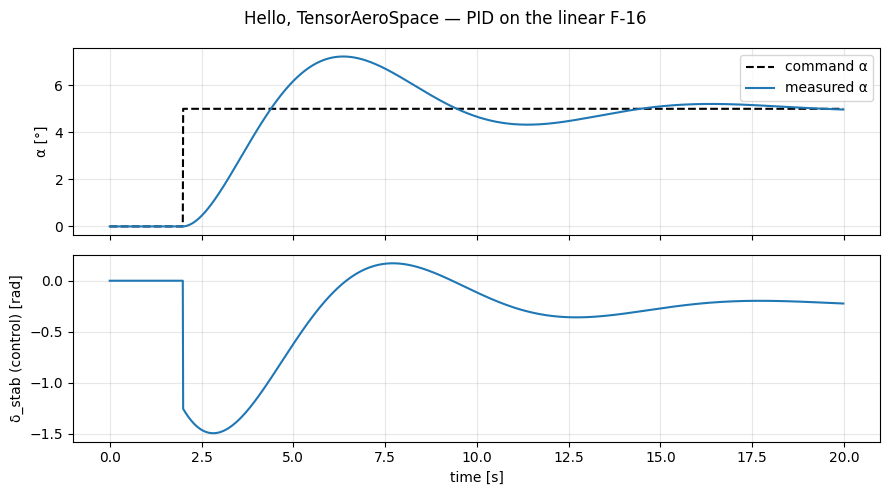
The top panel should show α reaching the 5° command within ~1 s and holding. The bottom panel shows the elevator command transient, settling to a small steady-state value.
Common mismatches
| Symptom | Likely cause |
|---|---|
| α stays near 0 | Positive PID gains (should be all negative for this plant). |
| α oscillates / diverges | Too large gain magnitudes, or dt in PID doesn't match env dt. |
| RMSE > 1° | tracking_states doesn't match the reference shape. |
IndexError near end of loop |
Loop goes to number_time_steps instead of number_time_steps - 2. |
Where to go next
- Recipe 02 — Anatomy of an env — every env argument explained.
- Recipe 03 — Crafting reference signals — beyond a single step.
- Recipe 04 — Choosing an agent — when PID is not enough.