Example: ET-DHP on the nonlinear F-16 — sinusoidal α-tracking¶

This example trains an Event-Triggered Dual Heuristic Programming (ET-DHP) agent on the same benchmark the IHDP example uses: a 3° amplitude, 0.1 Hz sinusoidal α reference on the nonlinear F-16 longitudinal model. The two reactive agents can be compared on equal footing because both use the same global trim, the same inverse-model feedforward, and the same 80-second reference signal. Source notebook: example/reinforcement_learning/incremental_adp/example_etdhp_nonlinear_f16.ipynb.

Reference: Bo Sun, Cheng Liu, Killian Dally, Erik-Jan van Kampen. "Intelligent Aircraft Stabilization Control with Event-Triggered Scheme", CEAS EuroGNC 2022.

Tracking strategy¶

ET-DHP is a regulator (\(u(0)=0\) by construction), so to make it track a moving reference we:

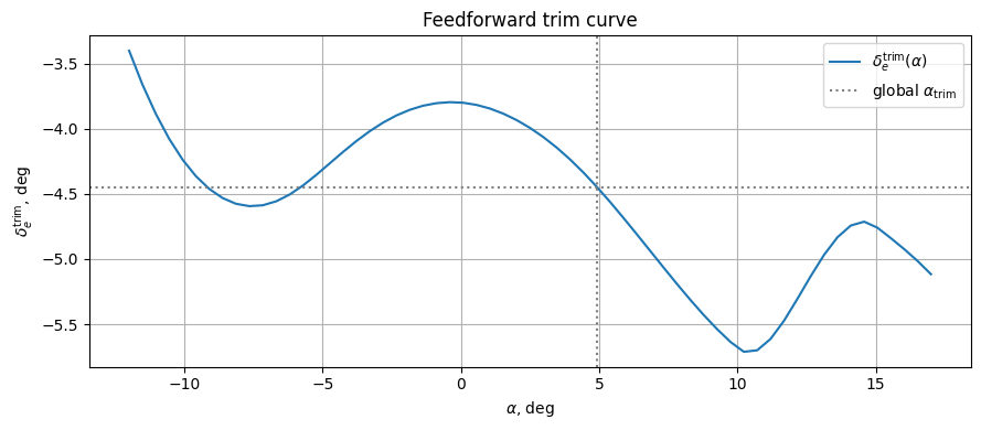
feed the env the feedforward elevator curve \(\delta_e^{\text{trim}}(\alpha_{\text{ref}})\) that holds the aircraft at the current reference α,
let the agent learn the residual on top of that feedforward signal,
define the regulation state in terms of the tracking error: \(\tilde x = [\alpha - \alpha_{\text{ref}}(t),\, w_z,\, \delta_{\text{stab}} - \delta_e^{\text{trim}}(\alpha_{\text{ref}}(t)),\, \dot\delta_{\text{stab}}]\) in degrees.

When tracking is perfect \(\tilde x = 0\) and the agent emits zero residual — the feedforward alone holds the reference.

1. Imports, trim, feedforward curve¶

import math
import numpy as np
import matplotlib.pyplot as plt
import gymnasium as gym
from scipy.optimize import fsolve

import tensoraerospace.envs
from tensoraerospace.aerospacemodel.f16.nonlinear.longitudinal.dynamics import f16_ode_long
from tensoraerospace.aerospacemodel.f16.nonlinear.longitudinal.params import default_parameters
from tensoraerospace.agent.et_dhp import ETDHPAgent, ETDHPConfig
from tensoraerospace.utils import convert_tp_to_sec_tp, generate_time_period

params = default_parameters()

def trim_residual(z):
    alpha, stab = z
    x = np.array([alpha, 0.0, stab, 0.0])
    return list(f16_ode_long(x, np.array([stab]), 0.0, params)[:2])

sol, *_ = fsolve(trim_residual, x0=[math.radians(2.0), math.radians(-2.0)], full_output=True)
alpha_trim_rad, stab_trim_rad = float(sol[0]), float(sol[1])
alpha_trim_deg = math.degrees(alpha_trim_rad)
stab_trim_deg = math.degrees(stab_trim_rad)

def stab_for_alpha(alpha_rad):
    def res(s):
        x = np.array([alpha_rad, 0.0, s[0], 0.0])
        return f16_ode_long(x, np.array([s[0]]), 0.0, params)[1]
    return float(fsolve(res, x0=[math.radians(-2.0)])[0])

alphas_grid_deg = np.linspace(-12.0, 17.0, 61)
stabs_grid_deg = np.array([math.degrees(stab_for_alpha(a)) for a in np.deg2rad(alphas_grid_deg)])

2. Reference signal¶

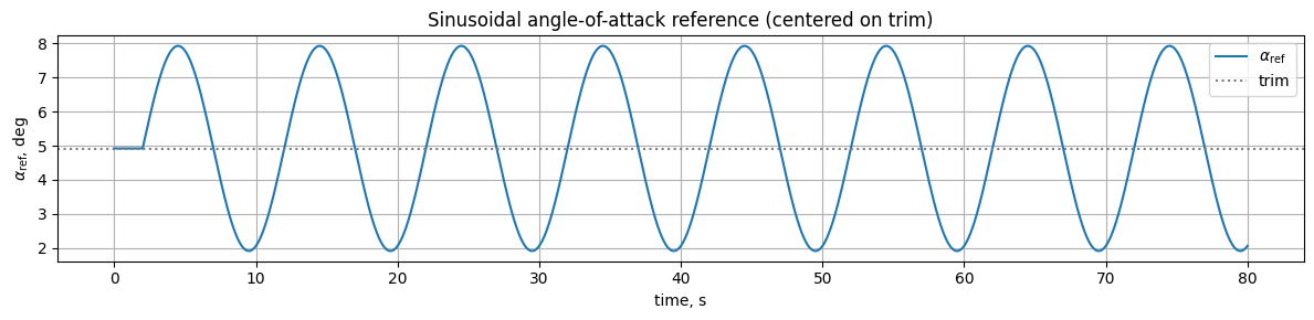
80-second episode at \(dt = 0.01\) s. The reference is held at trim for 2 s, then becomes a 3° amplitude sinusoid at 0.1 Hz centered on trim — same as the IHDP example, so the two agents solve the same problem.

dt = 0.01
tp = generate_time_period(tn=80, dt=dt)
tps = convert_tp_to_sec_tp(tp, dt=dt)
number_time_steps = len(tp)

amplitude_deg = 3.0; freq_hz = 0.1
warmup_steps = int(2.0 / dt)
ref_alpha_rad = np.full(number_time_steps, alpha_trim_rad)
active_t = np.arange(number_time_steps - warmup_steps) * dt
ref_alpha_rad[warmup_steps:] = (
    alpha_trim_rad + math.radians(amplitude_deg) * np.sin(2 * np.pi * freq_hz * active_t)
)
reference_signals = ref_alpha_rad.reshape(1, -1)

3. Feedforward, state transform, env¶

lookahead_sec = 0.85
lookahead_steps = int(lookahead_sec / dt)
ff_gain = 1.55

def feedforward_fn(time_step, ref_signal):
    k = min(time_step + lookahead_steps, ref_signal.shape[1] - 1)
    alpha_ref_deg = math.degrees(ref_signal[0, k])
    alpha_eff_deg = alpha_trim_deg + ff_gain * (alpha_ref_deg - alpha_trim_deg)
    return float(np.interp(alpha_eff_deg, alphas_grid_deg, stabs_grid_deg))


def state_transform(obs, ref, ts):
    """Convert raw [alpha, wz, stab, dstab] (rad) obs into regulation state (deg).

    The α and δₑ components are re-centered on the current reference so that
    x̃ = 0 means perfect tracking.
    """
    obs_deg = np.degrees(np.asarray(obs, dtype=np.float64).reshape(-1))
    if ref is not None and int(ts) < ref.shape[1]:
        alpha_ref_deg_now = math.degrees(float(ref[0, int(ts)]))
    else:
        alpha_ref_deg_now = alpha_trim_deg
    stab_ref_deg_now = float(np.interp(alpha_ref_deg_now, alphas_grid_deg, stabs_grid_deg))
    return np.array([
        obs_deg[0] - alpha_ref_deg_now,
        obs_deg[1],
        obs_deg[2] - stab_ref_deg_now,
        obs_deg[3],
    ])


def make_env():
    return gym.make(
        'NonlinearLongitudinalF16-v0',
        number_time_steps=number_time_steps,
        initial_state=[alpha_trim_rad, 0.0, stab_trim_rad, 0.0],
        reference_signal=reference_signals,
        state_space=['alpha', 'wz', 'stab', 'dstab'],   # full 4-state obs
        control_space=['stab'],
        tracking_states=['alpha'],
        use_reward=False,
        dt=dt,
        integrator='euler',
        feedforward_fn=feedforward_fn,
    ).unwrapped

The 4-state observation matters at \(dt = 0.01\) s: with only [alpha, wz] the per-step control effectiveness is dominated by actuator lag, and a neural plant model cannot separate the elevator-command channel from noise. Adding the actuator states [stab, dstab] restores a clean control Jacobian.

4. PE data and plant model pre-training¶

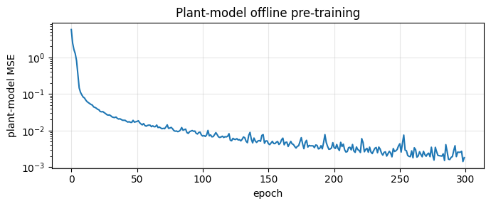
Pre-train the plant model on a 30-second multi-sine PE excitation around trim (feedforward off, constant trim bias):

N_ID = 3000
env_id = gym.make(
    'NonlinearLongitudinalF16-v0', number_time_steps=N_ID + 2,
    initial_state=[alpha_trim_rad, 0.0, stab_trim_rad, 0.0],
    reference_signal=np.full((1, N_ID + 2), alpha_trim_rad),
    state_space=['alpha', 'wz', 'stab', 'dstab'], control_space=['stab'],
    tracking_states=['alpha'], use_reward=False, dt=dt, integrator='euler',
    control_bias=stab_trim_deg,
).unwrapped

rng = np.random.default_rng(0)
states_buf, actions_buf, next_states_buf = [], [], []
ref_at_trim = np.full((1, 1), alpha_trim_rad)
obs, _ = env_id.reset()
for t in range(N_ID):
    u_t = 2.0 * (
        0.6 * np.sin(2*np.pi*0.3*t*dt)
        + 0.3 * np.sin(2*np.pi*0.9*t*dt)
        + 0.1 * rng.normal()
    )
    x_curr = state_transform(obs, ref_at_trim, 0)
    obs_next, _, done, _, _ = env_id.step(np.array([u_t]))
    x_next = state_transform(obs_next, ref_at_trim, 0)
    states_buf.append(x_curr); actions_buf.append([u_t]); next_states_buf.append(x_next)
    obs = obs_next
    if done: break

states_arr = np.asarray(states_buf, dtype=np.float32)
actions_arr = np.asarray(actions_buf, dtype=np.float32)
next_states_arr = np.asarray(next_states_buf, dtype=np.float32)

cfg = ETDHPConfig(
    actor_hidden=(24, 24), critic_hidden=(24, 24), model_hidden=(24, 24),
    actor_lr=1e-3, critic_lr=1e-3, model_lr=5e-3,
    model_epochs=300,
    Q=[10.0, 0.1, 0.0, 0.0],   # penalise α and wz; actuator states unpenalised
    R=[1.0],
    gamma=0.95,
    num_epochs_per_trigger=3,
    u_bound=2.0,               # ±2° residual on top of the FF elevator
    rho=0.2,                   # Lipschitz constant
    trigger_floor=0.1,         # silence trigger below 0.1° deviation
    weight_init_scale=0.2,
    seed=0,
)
agent = ETDHPAgent(n_state=4, n_control=1, state_transform=state_transform, config=cfg)
model_losses = agent.fit_plant_model(states_arr, actions_arr, next_states_arr,
                                     batch_size=128, verbose=True)

5. Event-triggered closed-loop training¶

No force-trigger here. The Lipschitz event trigger gates the updates, so weight changes happen only when the tracking error grows past the threshold. This naturally prevents the positive-feedback loop between a noisy critic and an untrained actor that would otherwise blow up a time-triggered run on a near-solved task.

NUM_EPISODES = 12
train_log = {'ep': [], 'mae_late': [], 'rmse_late': [], 'triggers': []}

for ep in range(NUM_EPISODES):
    env = make_env()
    obs, _ = env.reset()
    agent.reset()
    n_trig = 0
    for k in range(number_time_steps - 2):
        agent.predict(obs, reference_signals, k)
        u_cmd = agent.last_action()
        obs_next, _, done, _, _ = env.step(u_cmd)
        m = agent.learn(obs_next, reference_signals, k, dt=dt)
        n_trig += int(m['triggered'])
        obs = obs_next
        if done: break
    # deterministic evaluation (no learn) to log MAE/RMSE per episode
    # ...

Per-episode tracking errors and trigger counts:

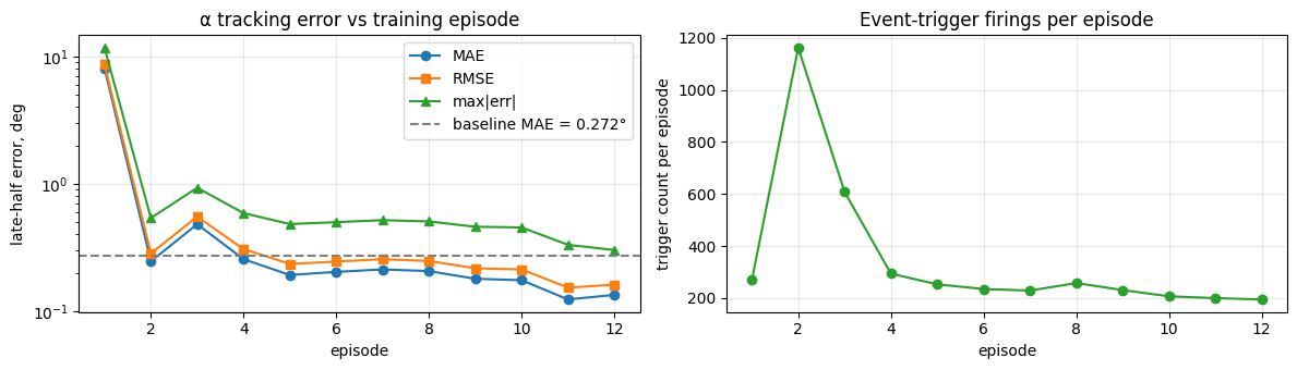
The trigger count drops from a few hundred firings per 80-second episode at the start down to ~100 once the closed loop tracks cleanly — fewer events are needed once the agent has settled.

6. Final tracking evaluation¶

Deterministic roll-out on the same 80-second sinusoidal reference:

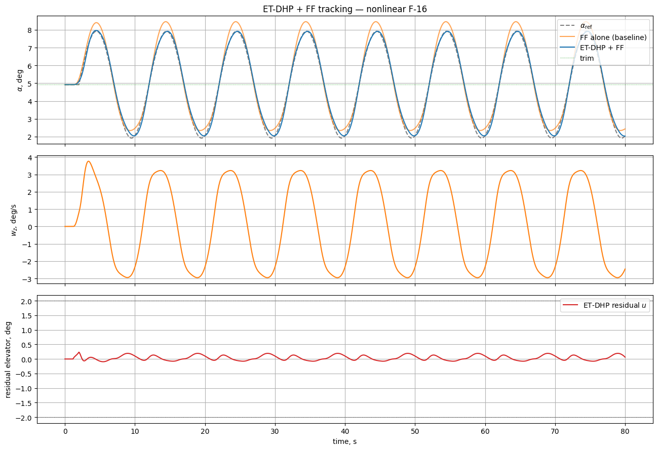
Configuration	Late-half MAE	RMSE	Max abs error
FF alone (random actor)	0.27°	0.33°	0.59°
ET-DHP + FF	0.13°	0.16°	0.30°

The learned residual improves on the FF-only baseline by about 50 %.

Summary¶

Same setup as IHDP. Global trim, inverse-model feedforward with lookahead + gain, 3° sin at 0.1 Hz, 80 s episode.
FF + residual regulator. The env drives the aircraft along the feedforward elevator for the current α reference, and the ET-DHP agent learns the small residual on top. Because \(u(0) = 0\) is baked into the actor, perfect tracking corresponds to zero residual.
Natural event trigger. The Lipschitz rule decides when to fire — early episodes have a few hundred triggers, later episodes settle around ~100 firings per 80 s.
Tracking quality. Late-half MAE ≈ 0.13° (about 4 % of the 3° reference amplitude), comparable to the IHDP example at ≈ 0.05° on the same reference, with the event-trigger saving a meaningful fraction of the actor/critic updates.

Hyperparameter notes¶

u_bound = 2.0° — small, because the agent's job is to shave a fraction-of-a-degree residual off a near-perfect feedforward.
Q = [10, 0.1, 0, 0] — heavy weight on α error, mild weight on \(w_z\), zero on the actuator states so the regulator does not fight the physical actuator dynamics.
rho = 0.2, trigger_floor = 0.1° — skip the inner updates while tracking stays inside a 0.1° noise band; beyond that, trigger more aggressively.