Recipe 03 — Crafting reference signals
Hands-on walk through the library's signal primitives, then composite schedules (doublets, multi-level holds, smoothed transitions). Copy each block and compare your plot with the reference plot below.
Source notebook: example/cookbook/recipe_03_reference_signals.ipynb.
Shape contract (read once)
The env expects reference_signal.shape == (len(tracking_states), number_time_steps). For one tracked channel always np.reshape(sig, (1, -1)). All library builders in tensoraerospace.signals.standard take the time vector tp = generate_time_period(tn=T, dt=dt) as the first argument.
Step 1 — Primitives
import warnings
warnings.filterwarnings('ignore')

import matplotlib.pyplot as plt
import numpy as np

from tensoraerospace.signals.standard import (
    unit_step, ramp, pulse, sinusoid, sinusoid_vertical_shift,
    square_wave, constant_line,
)
from tensoraerospace.utils import generate_time_period

dt = 0.01
tp = generate_time_period(tn=10, dt=dt)       # 10 s, 1001 ticks

fig, axes = plt.subplots(3, 2, figsize=(10, 7), sharex=True)
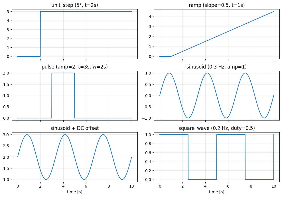
axes[0,0].plot(tp, unit_step(tp=tp, degree=5, time_step=2.0));            axes[0,0].set_title('unit_step (5°, t=2s)')
axes[0,1].plot(tp, ramp(tp=tp, slope=0.5, time_start=1.0));               axes[0,1].set_title('ramp (slope=0.5, t=1s)')
axes[1,0].plot(tp, pulse(tp=tp, amplitude=2.0, time_start=3.0, width=2.0)); axes[1,0].set_title('pulse')
axes[1,1].plot(tp, sinusoid(tp=tp, frequency=0.3, amplitude=1.0));         axes[1,1].set_title('sinusoid (0.3 Hz)')
axes[2,0].plot(tp, sinusoid_vertical_shift(tp=tp, frequency=0.3, amplitude=1.0, vertical_shift=2.0)); axes[2,0].set_title('sinusoid + DC offset')
axes[2,1].plot(tp, square_wave(tp=tp, frequency=0.2, amplitude=1.0));      axes[2,1].set_title('square_wave')
for ax in axes.flat: ax.grid(alpha=0.3)
plt.tight_layout(); plt.show()
Expected plot:
| Primitive | Signature |
|---|---|
unit_step |
(tp, degree, time_step, output_rad=False) |
ramp |
(tp, slope, time_start) |
pulse |
(tp, amplitude, time_start, width) |
sinusoid |
(tp, frequency, amplitude) |
sinusoid_vertical_shift |
(tp, frequency, amplitude, vertical_shift) |
square_wave |
(tp, frequency, amplitude, duty_cycle) |
constant_line |
(tp, value_state) |
Step 2 — Composite schedules
def doublet(tp, amplitude, t_start, half_width):
    return (pulse(tp=tp, amplitude=amplitude, time_start=t_start, width=half_width)
            + pulse(tp=tp, amplitude=-amplitude, time_start=t_start + half_width, width=half_width))

def multi_step(tp, schedule):
    """schedule: list of (t_start, level), sorted by time."""
    sig = np.zeros_like(tp)
    for i, (t_start, level) in enumerate(schedule):
        next_t = schedule[i+1][0] if i+1 < len(schedule) else tp[-1] + 1.0
        mask = (tp >= t_start) & (tp < next_t)
        sig[mask] = level
    return sig

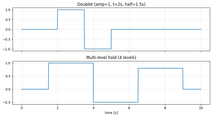
doublet_sig = doublet(tp, amplitude=1.0, t_start=2.0, half_width=1.5)
multi = multi_step(tp, [(0.0, 0.0), (1.5, 1.0), (4.0, -0.5), (6.5, 0.8), (9.0, 0.0)])

fig, axes = plt.subplots(2, 1, figsize=(9, 5), sharex=True)
axes[0].plot(tp, doublet_sig); axes[0].set_title('Doublet (amp=1, t=2s, half=1.5s)')
axes[1].plot(tp, multi); axes[1].set_title('Multi-level hold (4 levels)')
for ax in axes: ax.grid(alpha=0.3)
axes[1].set_xlabel('time [s]')
plt.tight_layout(); plt.show()
Expected plot:
When to use each:
- Doublet → frequency-response identification (aviation-standard excitation).
- Multi-level hold → batch LS policy evaluators (iADP etc.); different levels excite cross-terms of
P̃.
Step 3 — Smoothed transitions
Discontinuous steps excite everything up to actuator bandwidth — often nicer to soften them with tanh edges.
def smooth_step(tp, from_level, to_level, t_mid, transition_time):
    k = 4.0 / max(transition_time, 1e-6)
    return from_level + 0.5 * (to_level - from_level) * (1.0 + np.tanh(k * (tp - t_mid)))

smooth = (smooth_step(tp, 0.0, 1.0, t_mid=2.0, transition_time=1.0)
          + smooth_step(tp, 0.0, -1.5, t_mid=5.0, transition_time=1.0)
          + smooth_step(tp, 0.0, 0.5, t_mid=8.0, transition_time=1.0))

fig, ax = plt.subplots(figsize=(9, 3))
ax.plot(tp, smooth, label='smoothed')
ax.plot(tp, multi_step(tp, [(0.0, 0.0), (2.0, 1.0), (5.0, -0.5), (8.0, 0.5)]),
        alpha=0.4, label='hard step')
ax.set_xlabel('time [s]'); ax.set_ylabel('reference')
ax.legend(); ax.grid(alpha=0.3)
plt.tight_layout(); plt.show()
Expected plot:
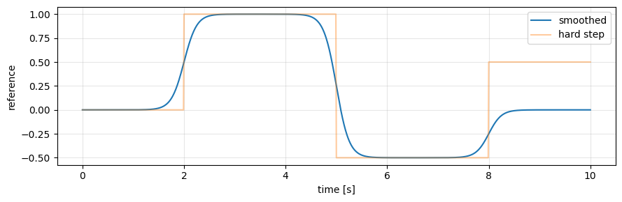
The hard step (faded line) switches levels instantaneously; the smoothed version (solid) ramps with transition_time = 1 s.
Step 4 — Feed into an env
One channel:
reference_signal = np.reshape(smooth, (1, -1))
env = gym.make('LinearLongitudinalF16-v0',
    number_time_steps=len(tp),
    reference_signal=reference_signal,
    tracking_states=['alpha'],
    ...)
Multi-channel (e.g. 6-DoF roll/pitch/yaw rates):
ref_p = doublet(tp, 0.3, 2.0, 1.0)
ref_q = smooth_step(tp, 0.0, 0.5, 4.0, 0.5)
ref_r = np.zeros_like(tp)
reference_signal = np.stack([ref_p, ref_q, ref_r], axis=0)
# tracking_states=['p', 'q', 'r']
Rules of thumb
- PID / MPC benchmarking — pulses and doublets.
- Adaptive-critic agents (IHDP / IM-GDHP / iADP) — multi-level hold.
- RL training — randomised schedules across episodes.
- Frequency-response ID — chirp or multi-sine. The iADP notebook uses
2·sin(2π·0.7t) + 1·sin(2π·1.5t).
Where to go next
- Recipe 04 — Choosing an agent — signal shape ↔ agent capability.
- Recipe 09 — Fault-tolerance — commands combined with actuator faults.