F‑16 Fighting Falcon — продольная динамика¶

General Dynamics F‑16 Fighting Falcon — американский многофункциональный лёгкий истребитель 4‑го поколения. В библиотеке реализован продольный канал полёта в виде линейной модели пространства состояний и соответствующей среды Gymnasium для обучения агентов управления.

Быстрый старт

Запустите среду или модель в пару строк кода.

К примеру
API модели

Документация Python‑класса продольной динамики F‑16.

К API
Среда Gymnasium

Готовая среда для обучения агентов управления.

К среде
Теория

Уравнения состояния и источники данных модели.

К модели

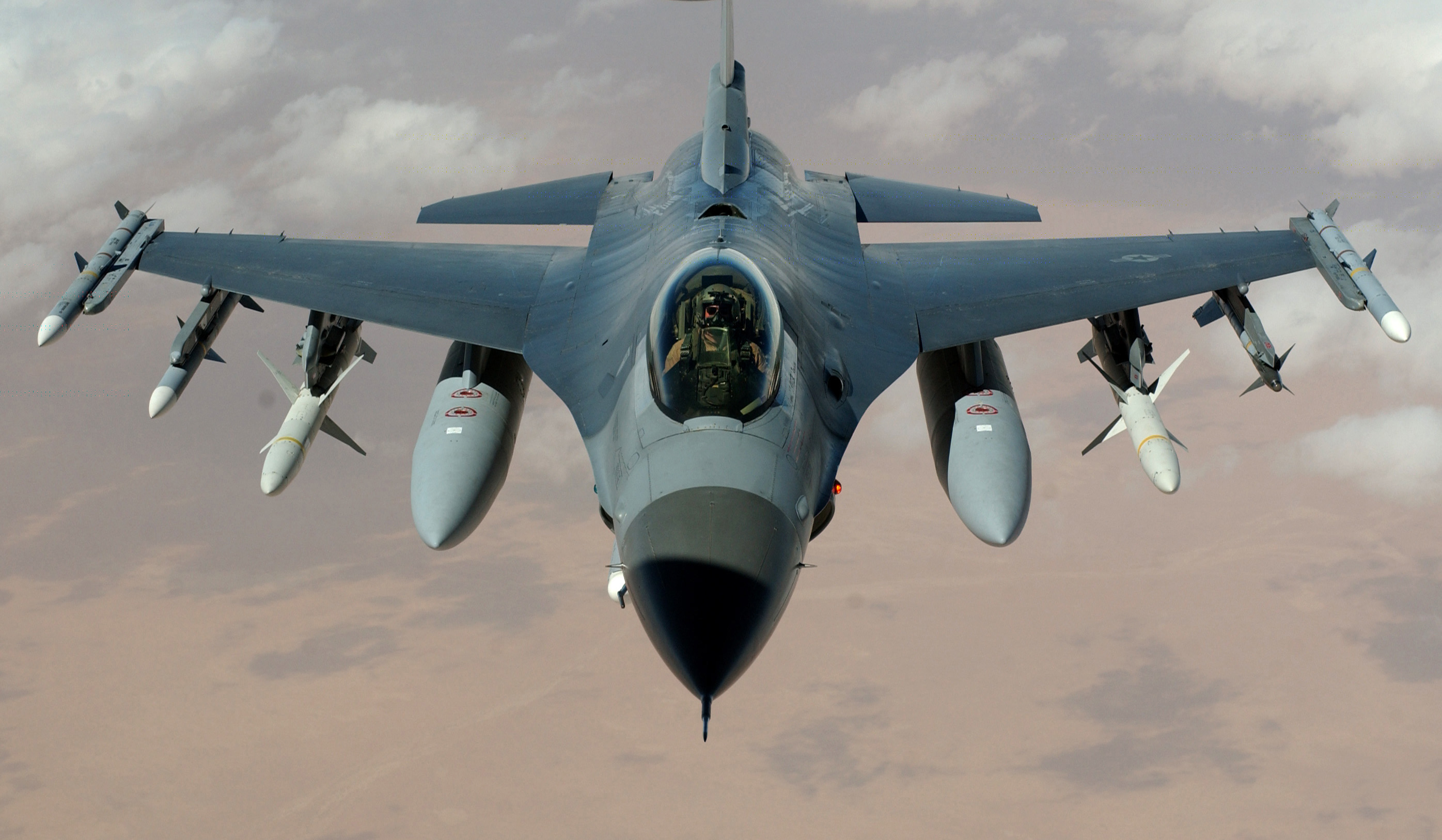
ЛТХ (справочно)¶

Параметр	Значение
Модификация	F‑16A Block 10
Размах крыла, м	9.45
Длина самолёта (со штангой ПВД), м	15.03
Высота самолёта, м	5.09
Площадь крыла, м²	27.87
Угол стреловидности, °	40.0
Нормальная взлётная масса, кг	11467

Как устроен объект управления¶

Модель задаётся в пространстве состояний и описывает эволюцию продольных переменных при управлении отклонением стабилизатора.

\[\dot{x} = A x + B u, \quad y = C x + D u\]

Где вектор состояния и управляющее воздействие выбраны как:

\[ x = \begin{bmatrix} u & \alpha & q & \theta \end{bmatrix}^{\top}, \quad u_{in} = \eta \]

Типичная структура матриц для продольного канала:

\[ \begin{bmatrix} \dot{u} \\ \dot{\alpha} \\ \dot{q} \\ \dot{\theta} \end{bmatrix} = \begin{bmatrix} x_u & x_{\alpha} & x_q & x_{\theta} \\ z_u & z_{\alpha} & z_q & z_{\theta} \\ m_u & m_{\alpha} & m_q & m_{\theta} \\ 0 & 0 & 1 & 0 \end{bmatrix} \begin{bmatrix} u \\ \alpha \\ q \\ \theta \end{bmatrix} + \begin{bmatrix} x_{\eta} \\ z_{\eta} \\ m_{\eta} \\ 0 \end{bmatrix} \eta \]

В используемой реализации параметры получены из источника ниже и редуцированы к выбранным переменным, после чего система дискретизируется с шагом dt.

ПеременныеКоэффициенты

u: продольная скорость, м/с
α: угол атаки, рад (в API доступны преобразования в градусы)
q: угловая скорость тангажа, рад/с
θ: тангаж, рад
η: управляющее отклонение стабилизатора, рад

x_u, x_α, x_q, x_θ: производные продольной силы
z_u, z_α, z_q, z_θ: производные нормальной силы (по принятым осям — строка Z)
m_u, m_α, m_q, m_θ: производные момента тангажа

О единицах измерения

Внутри моделей углы и угловые скорости задаются в радианах. Методы получения историй состояний/управлений поддерживают конвертацию в градусы.

Математическая модель¶

\[ \dot{x} = A x + B u, \qquad y = C x + D u \]

Так как объект управления представляет собой объект без внутренних возмущающих процессов, выход системы \(y\) не используется в моделировании (\(C\) — диагональная, \(D\) — нулевая матрица).

\[ \begin{bmatrix} \dot{u} \\ \dot{\alpha} \\ \dot{q} \\ \dot{\theta} \end{bmatrix} = \begin{bmatrix} -0.1656 & -10.7137 & -7.2815 & -32.1740 \\ -0.0018 & -0.0981 & 0.9276 & 0 \\ 0 & -0.6252 & -0.4673 & 0 \\ 0 & 0 & 1 & 0 \end{bmatrix} \begin{bmatrix} u \\ \alpha \\ q \\ \theta \end{bmatrix} + \begin{bmatrix} -4.0478 \\ -0.0253 \\ -0.8992 \\ 0 \end{bmatrix} \eta \]

Производные (численные значения)¶

Матрица A (производные):

Коэффициент	Значение
x_u	-0.1656
x_α	-10.7137
x_q	-7.2815
x_θ	-32.1740
z_u	-0.0018
z_α	-0.0981
z_q	0.9276
z_θ	0
m_u	0
m_α	-0.6252
m_q	-0.4673
m_θ	0

Вход η (столбец B):

Коэффициент	Значение
x_η	-4.0478
z_η	-0.0253
m_η	-0.8992

Расшифровка коэффициентов¶

x_u, x_α, x_q, x_θ — частные производные продольной силы \(X\) по переменным \(u, \alpha, q, \theta\) соответственно
z_u, z_α, z_q, z_θ — частные производные нормальной силы \(Z\) по переменным \(u, \alpha, q, \theta\)
m_u, m_α, m_q, m_θ — частные производные момента тангажа \(M\) по переменным \(u, \alpha, q, \theta\)
x_η, z_η, m_η — частные производные по управляющему воздействию \(\eta\) (отклонение стабилизатора)

где

\(u\) — продольная скорость ЛА [м/с]
\(\alpha\) — угол атаки [рад]
\(q\) — угловая скорость тангажа [рад/с]
\(\theta\) — тангаж [рад]
\(\eta\) — отклонение стабилизатора [рад]

Ограничения привода

По умолчанию в модели применяются предельные значения управления:

Максимальная величина: \(\pm 25^\circ\)
Максимальная скорость изменения: \(60^\circ/\text{s}\)

Внутренние вычисления ведутся в радианах; ограничения эквивалентно переводятся.

Источник данных¶

Albert Farré Gabernet, "Controllers for Systems with Bounded Actuators: Modeling and control of an F‑16 aircraft", University of California, Irvine. Ссылка

Быстрый старт¶

GymnasiumТолько модель

import gymnasium as gym
import numpy as np

from tensoraerospace.envs import LinearLongitudinalF16
from tensoraerospace.utils import generate_time_period
from tensoraerospace.signals.standard import unit_step

dt = 0.01
tp = generate_time_period(tn=20, dt=dt)
number_time_steps = len(tp)
reference_signal = unit_step(degree=5, tp=tp, time_step=10, output_rad=True).reshape(1, -1)

env = gym.make(
    'LinearLongitudinalF16-v0',
    number_time_steps=number_time_steps,
    initial_state=[[0],[0]],  # alpha, q
    reference_signal=reference_signal,
)

state, info = env.reset()
for _ in range(200):
    action = np.array([[0.1]])  # рад
    state, reward, terminated, truncated, info = env.step(action)
    if terminated or truncated:
        break

import numpy as np
from tensoraerospace.aerospacemodel.f16.linear.longitudinal.model import LongitudinalF16

dt = 0.01
number_time_steps = 200

# Порядок internal-состояний модели: [theta, alpha, q, ele]
x0 = np.array([0.0, 0.0, 0.0, 0.0])

model = LongitudinalF16(
    x0=x0,
    number_time_steps=number_time_steps,
    selected_state_output=["alpha", "q"],
    dt=dt,
)

for t in range(number_time_steps - 1):
    u = np.array([[0.1]])  # отклонение стабилизатора (рад)
    state_next = model.run_step(u)

Python API¶

МодельСреда Gymnasium

`LongitudinalF16(x0, number_time_steps, selected_state_output=None, t0=0, dt=0.01)` ¶

Bases: ModelBase

Linearized longitudinal F-16 dynamics in state space.

The model describes the longitudinal channel of the aircraft with input via stabilizer deflection and outputs via angles/velocities. State matrices are loaded from prepared MATLAB files and reduced to selected variables, then the system is discretized with step dt.

States (internal-model order): theta: pitch [rad] alpha: angle of attack [rad] q: pitch angular velocity [rad/s] ele: elevator position [rad]

Control

ele: stabilizer deflection [rad]

Parameters:

Name	Type	Description	Default
`x0`	`ndarray \| list[float]`	Initial model state in internal-model order (see list above).	required
`number_time_steps`	`int`	Number of simulation steps.	required
`selected_state_output`	`list[str] \| None`	Names of states that are returned externally (reduced state vector). If `None`, full internal-model vector is returned.	`None`
`t0`	`float`	Initial time, sec.	`0`
`dt`	`float`	Discretization step, sec.	`0.01`

Attributes:

Name	Type	Description
`selected_states`	`list[str]`	List of internal-model states.
`selected_output`	`list[str]`	List of outputs.
`selected_input`	`list[str]`	List of control inputs.
`input_magnitude_limits`	`list[float]`	Control magnitude limits.
`input_rate_limits`	`list[float]`	Control rate limits.
`A,`	`B, C, D (np.ndarray \| None`	Continuous matrices of original system.
`filt_A,`	`filt_B, filt_C, filt_D (np.ndarray \| None`	Filtered and discretized matrices of reduced system.
`store_states,`	`store_input, store_outputs (np.ndarray`	History of states, inputs and outputs over simulation horizon.

Notes

Matrices are loaded from the ../data directory relative to this file.
Discretization is performed using scipy.signal.cont2discrete.
Units: angles and angular rates inside the model are in radians.

`import_linear_system()` ¶

Load linearized state-space matrices from MATLAB files.

`simplify_system()` ¶

Reduce the system to selected states/outputs and form filtered matrices.

`create_dictionary(file_name)` ¶

Create a dictionary that maps quantity names to indices (state/input/output).

Parameters:

Name	Type	Description	Default
`file_name`	`str`	Key file name (`states`, `input`, `output`).	required

Returns:

Type	Description
`dict[str, int]`	dict[str, int]: Mapping from quantity name to row/column index.

`initialise_system(x0, number_time_steps)` ¶

Initialize the system, discretize it, and allocate history buffers.

Parameters:

Name	Type	Description	Default
`x0`	`ndarray`	Initial state.	required
`number_time_steps`	`int`	Simulation horizon.	required

`run_step(ut_0)` ¶

Perform one evolution step subject to control constraints.

Parameters:

Name	Type	Description	Default
`ut_0`	`ndarray`	Control vector at the current step (rad).	required

Returns:

Type	Description
`ndarray`	np.ndarray: Next-step state `x[t+1]`.

`update_system_attributes()` ¶

Update the current state and the internal model timer.

`get_state(state_name, to_deg=False, to_rad=False)` ¶

Get the state history array.

Parameters:

Name	Type	Description	Default
`state_name`	`str`	State name.	required
`to_deg`	`bool`	Convert to degrees.	`False`
`to_rad`	`bool`	Convert to radians.	`False`

Returns:

Type	Description
`ndarray`	History array of the selected state.

Example:

state_hist = model.get_state('alpha', to_deg=True)

`get_control(control_name, to_deg=False, to_rad=False)` ¶

Get the control signal history array.

Parameters:

Name	Type	Description	Default
`control_name`	`str`	Name of the control signal.	required
`to_deg`	`bool`	Convert to degrees.	`False`

Returns:

Type	Description
`ndarray`	History array of the selected control signal.

Example:

state_hist = model.get_control('stab', to_deg=True)

`LinearLongitudinalF16(initial_state, reference_signal, number_time_steps, tracking_states=None, state_space=None, control_space=None, output_space=None, reward_func=None, use_reward=True)` ¶

Bases: Env

Simulation of LongitudinalF16 control object in OpenAI Gym environment for training AI agents.

Parameters:

Name	Type	Description	Default
`initial_state`	`ndarray`	Initial state.	required
`reference_signal`	`ndarray`	Reference signal.	required
`number_time_steps`	`int`	Number of simulation steps.	required
`tracking_states`	`list[str] \| None`	Tracked states.	`None`
`state_space`	`list[str] \| None`	State space.	`None`
`control_space`	`list[str] \| None`	Control space.	`None`
`output_space`	`list[str] \| None`	Full output space (including noise).	`None`
`reward_func`	`Callable[[ndarray, ndarray, int], ndarray \| float] \| None`	Reward function (WIP status).	`None`

Initialize LinearLongitudinalF16 environment.

Parameters:

Name	Type	Description	Default
`initial_state`	`ndarray`	Initial state.	required
`reference_signal`	`ndarray`	Reference signal.	required
`number_time_steps`	`int`	Number of simulation steps.	required
`tracking_states`	`list`	Tracked states. Defaults to ["alpha", "q"].	`None`
`state_space`	`list`	State space. Defaults to ["alpha", "q"].	`None`
`control_space`	`list`	Control space. Defaults to ["ele"].	`None`
`output_space`	`list`	Full output space. Defaults to ["alpha", "q"].	`None`
`reward_func`	`callable`	Reward function. Defaults to None.	`None`
`use_reward`	`bool`	Whether to use reward. Defaults to True.	`True`

`get_init_args()` ¶

Get initialization arguments as a dictionary.

Returns:

Name	Type	Description
`dict`	`dict[str, object]`	Dictionary of initialization arguments.

`step(action)` ¶

Execute one simulation step.

Parameters:

Name	Type	Description	Default
`action`	`ndarray`	Control signal array for selected actuators.	required

Returns:

Name	Type	Description
`tuple`	`tuple[ndarray, float, bool, bool, dict[str, float]]`	Tuple containing: - next_state (np.ndarray): Next state of the control object. - reward (np.ndarray): Evaluation of control algorithm actions. - done (bool): Simulation status, whether completed or not. - truncated (bool): Whether episode was truncated. - info (dict): Additional information (not used).

`reset(seed=None, options=None)` ¶

Reset simulation environment to initial conditions.

Parameters:

Name	Type	Description	Default
`seed`	`int`	Random seed. Defaults to None.	`None`
`options`	`dict`	Reset options. Defaults to None.	`None`

Returns:

Name	Type	Description
`tuple`	`tuple[ndarray, dict[str, float]]`	Tuple containing: - observation (np.ndarray): Initial observation. - info (dict): Additional information.

`close()` ¶

Release resources (no-op placeholder).

`default_reward(state, ref_signal, ts)` `staticmethod` ¶

Reward function for RL environment in longitudinal aircraft control.

Supports variable-length state vectors. The last two elements of the flattened state are treated as [tracked_angle, angular_rate] so the reward works for both 2-state [alpha, q] and 3-state [theta, alpha, q] configurations.

Parameters:

Name	Type	Description	Default
`state`	`ndarray`	Current aircraft state (at least 2 elements).	required
`ref_signal`	`ndarray`	Target angle trajectory, shape `(1, T)`.	required
`ts`	`int`	Current time step index.	required

Returns:

Type	Description
`ndarray`	np.ndarray: Reward value for this step.

F‑16 Fighting Falcon — продольная динамика¶

ЛТХ (справочно)¶

Как устроен объект управления¶

Математическая модель¶

Производные (численные значения)¶

Расшифровка коэффициентов¶

Источник данных¶

Быстрый старт¶

Python API¶

LongitudinalF16(x0, number_time_steps, selected_state_output=None, t0=0, dt=0.01) ¶

import_linear_system() ¶

simplify_system() ¶

create_dictionary(file_name) ¶

initialise_system(x0, number_time_steps) ¶

run_step(ut_0) ¶

update_system_attributes() ¶

get_state(state_name, to_deg=False, to_rad=False) ¶

get_control(control_name, to_deg=False, to_rad=False) ¶

LinearLongitudinalF16(initial_state, reference_signal, number_time_steps, tracking_states=None, state_space=None, control_space=None, output_space=None, reward_func=None, use_reward=True) ¶

get_init_args() ¶

step(action) ¶

reset(seed=None, options=None) ¶

close() ¶

default_reward(state, ref_signal, ts) staticmethod ¶

`LongitudinalF16(x0, number_time_steps, selected_state_output=None, t0=0, dt=0.01)` ¶

`import_linear_system()` ¶

`simplify_system()` ¶

`create_dictionary(file_name)` ¶

`initialise_system(x0, number_time_steps)` ¶

`run_step(ut_0)` ¶

`update_system_attributes()` ¶

`get_state(state_name, to_deg=False, to_rad=False)` ¶

`get_control(control_name, to_deg=False, to_rad=False)` ¶

`LinearLongitudinalF16(initial_state, reference_signal, number_time_steps, tracking_states=None, state_space=None, control_space=None, output_space=None, reward_func=None, use_reward=True)` ¶

`get_init_args()` ¶

`step(action)` ¶

`reset(seed=None, options=None)` ¶

`close()` ¶

`default_reward(state, ref_signal, ts)` `staticmethod` ¶